1.2 Row Operations
We need to learn how to row-reduce matrices. Row-reducing is a skill will use in almost every process and application problem in the first three-quarters of this course. Let’s begin with the matrix equation: \(A\vec x=\vec v\) where:
We need to first create MATLAB versions of the example matrix and the vector.
A=[0 0 -2 ; 2 0 -10 ; 1 1 -3]
v=[-4 ; 2 ; 3]
A =

     0     0    -2
     2     0   -10
     1     1    -3


v =

    -4
     2
     3
Matlab treats \(\vec v\) as a \(3\times 1\) matrix, and all built-in Matlab matrix operations work for vectors just as they do for marices.
Augmented Matrices
The solution vector \(\vec x\) can be found by row-reducing the corresponding augmented matrix:
We create the augmented matrix in Matlab using the code block below. The brackets say “join these two matrices into one” which MATLAB will do if its possible.
B=[A,v]
B =

     0     0    -2    -4
     2     0   -10     2
     1     1    -3     3
Now the column vector \(\vec v\) is the fourth column of the matrix. To refer to individual elements of matrix , we can specify its row and column:
To refer to an entire row (or column), we use a colon which is Matlab’s indexing operator:
B(2,:)
ans =

     2     0   -10     2
With the colon is in the column position, all elements in Row 2 are displayed as Matlab indexes through columns 1 through 4. We will use this indexing feature to create row operations.
Row Operations
We can use just the following three elementary row operations to solve any linear system:
Swapping two rows
Multiplying a row by a non-zero scalar
Replacing any row with the sum of that row and a scalar multiple of another row
Strategic Goal: Row Echelon Form


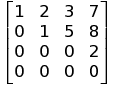
Examples of matrices in row-reduced form, abbreviated ref.
We have two ways to solve a linear system, a partial row-reduction method with back-substitution, and a full row-reduction method that leaves the solution on the right-hand side of the augmentation bar. The first step is to row-redcue to ref form
Row Operation 1: Swapping Rows
In the augmented matrix B, we see that Row 2 has a pivot in the third position. Thus, we can make progress by swapping Row 1 and Row 2.
B([2 1],:)=B([1 2],:)
B =

     2     0   -10     2
     0     0    -2    -4
     1     1    -3     3
Tip
We can swap multiple rows at once.
We would actually prefer the row starting with “1” to be our pivot, and we want the row that starts with zeros at the bottom. Let’s do all that at once with a multi-row-swap.
B([1 2 3],:)=B([3 1 2],:)
B =

     1     1    -3     3
     2     0   -10     2
     0     0    -2    -4
To understand the mapping, remember that the “old” matrix, the one we started with, is on the right side of the equal sign. The new matrix we are creating is on the left. Row 2 is sent to Row 1, Row 3 to Row 2 and Row 1 to Row 3.
b = B
b =

     1     1    -3     3
     2     0   -10     2
     0     0    -2    -4
Hint
Save your matrix into a new matrix before operating on it. This creates a saved checkpoint of your matrix. If you mess up later, you can return to this point rather than going all the way back to the beginning.
As you can in the above example, the lists in the brackets control how the rows will be swapped. Experiment with different values, and see what happens.
Row Operation 2: Multiplying a Row by a Non-zero Scalar
Let’s return to matrix B. Multiplying through the first row by \(-\frac{1}{2}\) will turn the first pivot into a one:
b(2,:) = b(2,:) / (-2)
b =

     1     1    -3     3
    -1     0     5    -1
     0     0    -2    -4
Pro Tip
Use lower case letters for matrices while performing row operations. They are a whole lot easier to type. Now \(B\) will be our clean copy of the original augmented matrix, and we can keep working with \(b\).
Let’s do the same with Row 3: multiply through by \(-\frac{1}{2}\). While neither of these row operations are needed, when working by we often multiply through a row by a non-zero real to make life easier.
b(3,:) = b(3,:) / (-2)
b =

     1     1    -3     3
    -1     0     5    -1
     0     0     1     2
Row Operation 3: Replacing a Row with the Sum of that Row and a Scalar Multiple of Another Row
Pro Tip
This is the workhorse row op – learn it well, grasshopper.
We would now like to replace Row subtract Row 2 minus Row 1:
so that entry , and thus we will have all zeros below the first pivot:
b(2,:)=b(2,:)+b(1,:)
b =

     1     1    -3     3
     0     1     2     2
     0     0     1     2
REF Completed
If we wish to solve the linear system, often the fastest way is using back substitution, with “back” indicating we start from the bottom-right and work our way back up to the top-left. Think about the matrix \(b\) means in terms of algebraic equations.
The bottom row means
which implies the row above it simplifies to
so \(y = -2\). With these two values, we can solve for \(x\):
We now know that
is the solution vector.
Goal 2: Row-Reduce to RREF
First, let’s create a saved checkpoint, since all of our steps up to this point are correct.
c=b
c =

     1     1    -3     3
     0     1     2     2
     0     0     1     2
To make our way to RREF, we need get zeros above the “1” in the third row.
c(2,:)=c(2,:) - 2 * c(3,:)
c =

     1     1    -3     3
     0     1     0    -2
     0     0     1     2
And to get the zero in Row 1:
c(1,:)= c(1,:) + 3 * c(3,:)
c =

     1     1     0     9
     0     1     0    -2
     0     0     1     2
We want the element \(a_{12}=0\), so
c(1,:)= c(1,:) - c(2,:)
c =

     1     0     0    11
     0     1     0    -2
     0     0     1     2
Since the matrix is now in RREF, the solution is just the vector on the right side of the agumentation bar. To check our solution (beyond comparing it to back-substitution), we need a Matlab version of :
x=c(:,4)
x =

    11
    -2
     2
We can verify that as required:
A*x
v
ans =

    -4
     2
     3


v =

    -4
     2
     3
We can also use a logical operator to check:
A*x == v
ans =

  3x1 logical array

   1
   1
   1
If the two expressions were not equal, we would get an array of zero’s instead. We can also check whether our has produced the correct RREF by the using function RREF.
rref([A,v])
ans =

     1     0     0    11
     0     1     0    -2
     0     0     1     2
Warning
MATLAB does not have an REF function.
Hence, we have verified that we have the correct solution.
Examples
In the examples below, you can copy the code blocks into MATLAB. When you execute them, all the steps will be shown down to ref.
By-hand Examples
You should definitely learn to do row-reduction by hand. The first set of examples are great. They either have very few steps, or very easy calculations in every step, or both.
Example 1
A = [ 0     0     0     1 ;
      0     6     7     4;
      1     4    -2    -2 ;
      0     3     1     1  ]
b=A;
b([1 2 3 4],:) = b([3 4 2 1],:)
b(3,:) = b(3,:) - 2 * b(2,:)
Example 2
B = [ 1 0 ; -2 1 ; 2 -1 ; -2 1 ]
c = B;
c(2,:) = c(2,:) + 2 * c(1,:)
c(3,:) = c(3,:) - 2 * c(1,:)
c(4,:) = c(4,:) + 2 * c(1,:)
c(3,:) = c(3,:) + c(2,:)
c(4,:) = c(4,:) + c(2,:)