1. Analyzing Data using Personality Variables¶

from datascience import *
import numpy as np

%matplotlib inline
import matplotlib.pyplot as plots
plots.style.use('fivethirtyeight')

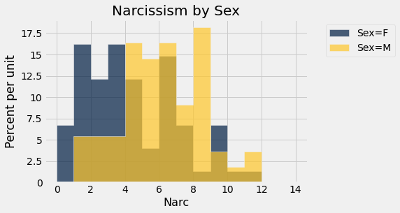
I keep some data frames in CSV format accessible from my website. One of them is called personality.csv and has, as you might imagine, personality variables. In this case, we will compare the narcissism levels based upon the grouping variable of biological sex.

pers = Table.read_table('http://faculty.ung.edu/rsinn/personality.csv')
pers.num_rows

pers.labels

('Age',
 'Yr',
 'Sex',
 'G21',
 'Corps',
 'Res',
 'Greek',
 'VarsAth',
 'Honor',
 'GPA',
 'Sleep',
 'Caff',
 'SitClass',
 'AccDate',
 'Friends',
 'TxRel',
 'Stress1',
 'Stress2',
 'CHS',
 'Thrill',
 'Eat',
 'TypeA',
 'Anx',
 'Opt',
 'SE',
 'Neuro',
 'Perf',
 'OCD',
 'Play',
 'Extro',
 'Narc',
 'HSAF',
 'HSSE',
 'HSAG',
 'HSSD',
 'PHS')

pers

Age	Yr	Sex	G21	Corps	Res	Greek	VarsAth	Honor	GPA	Sleep	Caff	SitClass	AccDate	Friends	TxRel	Stress1	Stress2	CHS	Thrill	Eat	TypeA	Anx	Opt	SE	Neuro	Perf	OCD	Play	Extro	Narc	HSAF	HSSE	HSAG	HSSD	PHS
21	2	M	Y	Y	1	N	N	N	3.23	3.5	2	F	N	O	25	15	10	28	23	45	31	30	27	61	29	105	10	142	8	11	41	40	26	27	SE
20	3	F	N	N	2	Y	N	Y	3.95	5.5	1	M	Y	E	15	13	11	29	25	32	32	37	23	60	44	105	3	172	16	11	46	52	26	33	SE
22	3	M	Y	N	2	N	N	N	3.06	8.5	1	B	Y	E	23	8	15	30	27	14	25	24	27	62	17	73	1	134	15	11	48	42	44	29	AG
27	3	F	Y	N	3	N	N	N	2.84	7	1	M	N	E	20	6	13	27	21	33	29	35	26	65	18	90	9	160	16	10	51	51	23	19	SE
24	3	M	Y	N	2	N	N	N	2.39	6	1	F	N	E	25	6	18	24	30	43	31	27	29	65	11	95	5	166	14	10	56	46	27	20	AF
22	3	F	Y	N	2	Y	N	N	2.63	6.5	0	F	N	E	18	17	12	16	26	39	31	34	20	68	43	114	20	133	10	9	40	27	31	28	AG
18	1	M	N	Y	1	N	N	N	3.17	6	3	M	Y	E	23	18	14	29	26	21	36	40	26	64	16	49	20	114	10	9	56	45	41	38	AG
20	3	F	N	N	1	Y	N	N	3.3	10	0	F	Y	E	22	16	17	29	17	42	32	41	21	50	45	142	17	168	16	9	55	45	24	29	AF
22	2	F	Y	N	1	N	N	N	3.02	3	6	B	N	O	24	18	18	31	21	42	30	58	8	45	73	119	16	141	10	9	52	47	32	26	SE
20	3	F	N	N	2	Y	N	N	3.22	3	0	M	N	E	20	14	14	20	18	42	36	43	17	60	54	117	16	136	5	9	34	32	32	32	AG

... (119 rows omitted)

narc = pers.select('Sex','Narc')

The nan value indicates there is no value for that cell in the table. In this case, it’s a survey item that went unanswered. The numpy function nanmean takes the average but ignores any nan values. In a clean table, we could just use np.mean, instead.

narc.group('Sex', np.nanmean)

Sex	Narc nanmean
F	3.94595
M	5.69091

integer_bins = np.arange(15)
narc.hist('Narc', group = "Sex", bins = integer_bins)
_=plots.title('Narcissism by Sex')

C:\Users\robbs\anaconda3\envs\datasci\lib\site-packages\datascience\tables.py:920: VisibleDeprecationWarning: Creating an ndarray from ragged nested sequences (which is a list-or-tuple of lists-or-tuples-or ndarrays with different lengths or shapes) is deprecated. If you meant to do this, you must specify 'dtype=object' when creating the ndarray.
  values = np.array(tuple(values))

males_narcissism = narc.where('Sex',"M").column('Narc')

females_narcissism = narc.where('Sex',"F").column('Narc')

print('The average narcissism level for males is',
      np.round(np.nanmean(males_narcissism),2),
      "\r\n",
      'and the average narcissism level for females is', 
      np.round(np.nanmean(females_narcissism),2)
     )

The average narcissism level for males is 5.69 
 and the average narcissism level for females is 3.95

from scipy import stats

stats.ttest_ind(males_narcissism, females_narcissism, axis=0, 
                equal_var=True, 
                nan_policy='omit', 
                alternative='two-sided')

Ttest_indResult(statistic=3.741532206524153, pvalue=0.00027577173246558825)

Intro to Applied Statistics

1. Analyzing Data using Personality Variables¶