25. Bootstrapping Examples
from datascience import *
import numpy as np

%matplotlib inline

import matplotlib.pyplot as plots
plots.style.use('fivethirtyeight')

from scipy import stats
Bootstrapping functions
The function boot_one creates a single resample and find its average. The function boot_hist takes an array representing a bootstrap distribution, plots it and calculates the 95% confidence interval.
def boot_one(table, samp_size):
    resample = table.sample(samp_size)
    return np.average(resample.column(0))
def boot_hist (array):
    left = round(percentile(2.5, array),2)
    right = round(percentile(97.5, array),2)
    avg = round(np.average(array),2)
    tab = Table().with_column('Bootstrapped Sample',array)
    tab.hist(0)
    _ = plots.title('95% Confidence Interval')
    _ = plots.plot([left, left], [0, 0.1], color='red', lw=2)
    _ = plots.plot([right, right], [0, 0.1], color='red', lw=2)
    _ = plots.scatter(avg, 0, color="gold", s = 200,zorder=2);
    print("The 95% confidence interval lies between ", left," and ", right, ",")
    print("and the gold dot at x = ", avg, " is the mean of the bootstrapped sample distribution.")
Often, creating a 90% confidence interval is useful. The code block below is indentical to the above except that it finds a 90% confidence interval instead.
def boot_hist_90 (array):
    left = round(percentile(5, array),2)
    right = round(percentile(95, array),2)
    avg = round(np.average(array),2)
    tab = Table().with_column('Bootstrapped Sample',array)
    tab.hist(0)
    _ = plots.title('90% Confidence Interval')
    _ = plots.plot([left, left], [0, 0.1], color='red', lw=2)
    _ = plots.plot([right, right], [0, 0.1], color='red', lw=2)
    _ = plots.scatter(avg, 0, color="gold", s = 200,zorder=2);
    print("The 90% confidence interval lies between ", left," and ", right, ",")
    print("and the gold dot at x = ", avg, " is the mean of the bootstrapped sample distribution.")
pers = Table.read_table('http://faculty.ung.edu/rsinn/perfnarc.csv')
pers.show(5)
| Sex | G21 | Greek | AccDate | Stress1 | Stress2 | Perf | Narc |
|---|---|---|---|---|---|---|---|
| F | N | N | N | 9 | 7 | 99 | 3 |
| F | Y | N | Y | 11 | 13 | 86 | 2 |
| F | N | Y | N | 15 | 14 | 118 | 4 |
| F | N | N | Y | 16 | 15 | 113 | 2 |
| F | Y | N | Y | 17 | 17 | 107 | 8 |
... (143 rows omitted)
Example 1: Narcissism
Estimate the average naricissism level for females undergraduates at UNG. We need to create a table with the correct numeric variable in the first column.
fem_narc = pers.where('Sex','F').select('Narc')
fem_narc.show(5)
| Narc |
|---|
| 3 |
| 2 |
| 4 |
| 2 |
| 8 |
... (80 rows omitted)
boot_samp = make_array()
resamp_size = 50

# Never need more than 1k reps, use 500 or fewer if working the cloud.
resample_reps = 1000

for i in range(resample_reps):
    new_boot = boot_one(fem_narc,resamp_size)
    boot_samp = np.append(boot_samp, new_boot)

# Remove the hashtag comment symbol to see the boot_samp results array
#boot_samp
boot_hist(boot_samp)
The 95% confidence interval lies between  3.1  and  4.56 ,
and the gold dot at x =  3.81  is the mean of the bootstrapped sample distribution.

Example 2: Prestest Stress
Let’s create two bootstrap confidence interval, one for pretest Stress (measured 2nd week of classes), one for posttest Stress (measured 7th week).
pre = pers.select('Stress1')
pre.show(5)
| Stress1 |
|---|
| 9 |
| 11 |
| 15 |
| 16 |
| 17 |
... (143 rows omitted)
boot_one(pre,50)
12.74
boot_samp_pre = make_array()
resamp_size = 50

# Never need more than 1k reps, use 500 or fewer if working the cloud.
resample_reps = 1000

for i in range(resample_reps):
    new_boot = boot_one(pre,resamp_size)
    boot_samp_pre = np.append(boot_samp_pre, new_boot)

# Remove the hashtag comment symbol to see the boot_samp results array
# boot_samp_pre
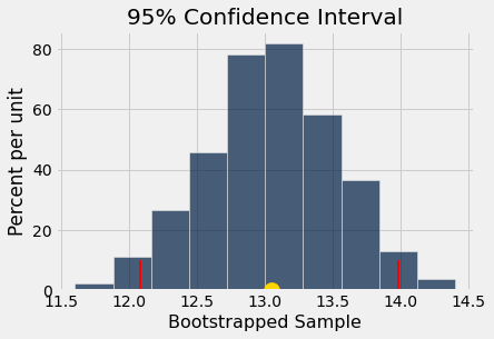
boot_hist(boot_samp_pre)
The 95% confidence interval lies between  12.08  and  13.98 ,
and the gold dot at x =  13.05  is the mean of the bootstrapped sample distribution.
Example 2b: Posttest Stress
Let’s compare the boostrap distributions from Pre and Post.
post = pers.select('Stress2')
post.show(5)
| Stress2 |
|---|
| 7 |
| 13 |
| 14 |
| 15 |
| 17 |
... (143 rows omitted)
boot_samp_post = make_array()
resamp_size = 50

# Never need more than 1k reps, use 500 or fewer if working the cloud.
resample_reps = 1000

for i in range(resample_reps):
    new_boot = boot_one(pre,resamp_size)
    boot_samp_post = np.append(boot_samp_post, new_boot)

# Remove the hashtag comment symbol to see the boot_samp results array
# boot_samp_pre
boot_hist(boot_samp_post)
The 95% confidence interval lies between  12.08  and  13.98 ,
and the gold dot at x =  13.03  is the mean of the bootstrapped sample distribution.
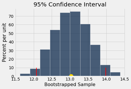
Comparing the bootstrap confidence intervals is like conducting an A/B test. Because the 95% confidence intervals overlap, we fail to the reject the null hypothesis at the 0.05 level. However, this is paired data. It would be interesting to bootstrap the gain score distribution to see typical gains are greater than zero.
gain_array = pers.select('Stress2').column(0) - pers.select('Stress1').column(0)
gain = Table().with_column('Gain',gain_array)
gain.show(5)
| Gain |
|---|
| -2 |
| 2 |
| -1 |
| -1 |
| 0 |
... (143 rows omitted)
boot_one(gain,len(gain))
4.0
boot_samp_gain = make_array()
resamp_size = 50

# Never need more than 1k reps, use 500 or fewer if working the cloud.
resample_reps = 1000

for i in range(resample_reps):
    new_boot = boot_one(gain, resamp_size)
    boot_samp_gain = np.append(boot_samp_gain, new_boot)

# Remove the hashtag comment symbol to see the boot_samp results array
# boot_samp_gain
boot_hist_90(boot_samp_gain)
The 90% confidence interval lies between  0.08  and  1.58 ,
and the gold dot at x =  0.84  is the mean of the bootstrapped sample distribution.
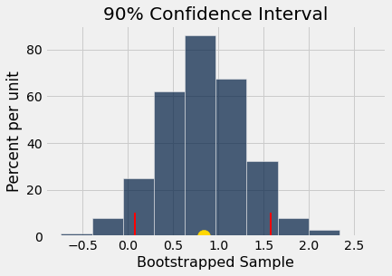
Since the 90% confidence interval does not include zero, we can conclude that the Gain in the Stress variable is positive. This result is analogous to a one-tailed pre-post hypothesis test at the 0.05 level of significance.