23. A/B Testing a Category Variable with 2 Levels
from datascience import *
import numpy as np

%matplotlib inline

import matplotlib.pyplot as plots
plots.style.use('fivethirtyeight')

from scipy import stats
We will continue to work with a subset of the personality table called pers. This time, however, we will focus on a category variable AccDate the responses to which are Yes/No based on this question. “At a time in your life when you are not involved with anyone, someone asks you out. This person has a great personality, but you do not find this person physically attractive. Do you accept the date?”
For the special case of a category variable with only two levels, we can use A/B testing. Since the test statistic is slightly different, the process will be quite similar to but not exactly like typical A/B tests with numeric variables.
pers = Table.read_table('http://faculty.ung.edu/rsinn/perfnarc.csv')
pers.show(5)
| Sex | G21 | Greek | AccDate | Stress1 | Stress2 | Perf | Narc |
|---|---|---|---|---|---|---|---|
| F | N | N | N | 9 | 7 | 99 | 3 |
| F | Y | N | Y | 11 | 13 | 86 | 2 |
| F | N | Y | N | 15 | 14 | 118 | 4 |
| F | N | N | Y | 16 | 15 | 113 | 2 |
| F | Y | N | Y | 17 | 17 | 107 | 8 |
... (143 rows omitted)
date = pers.select('Sex','AccDate')
date
| Sex | AccDate |
|---|---|
| F | N |
| F | Y |
| F | N |
| F | Y |
| F | Y |
| F | N |
| F | N |
| F | Y |
| F | Y |
| F | Y |
... (138 rows omitted)
Does biological sex affect Yes/No response to dating question?
A pivot table is the perfect data summary to reflect the difference in responses based on biological sex.
date.pivot('AccDate','Sex')
C:\Users\robbs\anaconda3\envs\datasci\lib\site-packages\datascience\tables.py:920: VisibleDeprecationWarning: Creating an ndarray from ragged nested sequences (which is a list-or-tuple of lists-or-tuples-or ndarrays with different lengths or shapes) is deprecated. If you meant to do this, you must specify 'dtype=object' when creating the ndarray.
  values = np.array(tuple(values))
| Sex | N | Y |
|---|---|---|
| F | 33 | 52 |
| M | 31 | 32 |
Steps in the hypothesis test
Null hypothesis. The grouping variable is independent of the response variable.
Alternate hypothesis. The response variable depends upon the grouping variable.
Test statistic. Simulated number of female Yes responses.
Simulate test statistic distribution with sample of 85 responses drawn without replacement.
Calculate \(p\)-value, e.g. the probability the null hypothesis is true.
Statistical Conclusion. If \(p<0.05\), reject null. Else, fail to reject null.
Real world implications. State the results of hypothesis test in real world terms.
Simulating the null hypothesis
The null hypothesis is that a person’s Yes/No response to the dating question is independent of their biological sex. There are 85 female responses. If sex has no bearing on the response, then repeated random draws of 85 responses should reveal whether 52 Yes responses in that group is typical.
As with the ab_shuffle function for A/B testing, the draws must be without replacement.
date.sample(85, with_replacement = False)
| Sex | AccDate |
|---|---|
| M | N |
| F | N |
| F | Y |
| F | N |
| F | Y |
| M | N |
| M | N |
| F | Y |
| M | N |
| F | Y |
... (75 rows omitted)
Our plan is to draw 85 random responses (without replacement) and record the number of Yes responses ignoring biological sex.
new_samp = date.sample(85, with_replacement = False).column(1)
new_samp
array(['Y', 'N', 'N', 'Y', 'N', 'N', 'Y', 'N', 'N', 'Y', 'Y', 'Y', 'Y',
       'N', 'N', 'Y', 'N', 'N', 'N', 'N', 'N', 'N', 'Y', 'Y', 'Y', 'N',
       'Y', 'Y', 'N', 'N', 'N', 'Y', 'N', 'Y', 'N', 'Y', 'Y', 'Y', 'Y',
       'Y', 'N', 'Y', 'N', 'N', 'Y', 'N', 'Y', 'Y', 'Y', 'Y', 'Y', 'Y',
       'N', 'Y', 'N', 'N', 'N', 'N', 'Y', 'N', 'Y', 'Y', 'Y', 'N', 'N',
       'N', 'Y', 'Y', 'Y', 'N', 'Y', 'Y', 'N', 'Y', 'Y', 'Y', 'N', 'N',
       'Y', 'N', 'Y', 'Y', 'Y', 'N', 'Y'], dtype='<U1')
sum(new_samp == 'Y')
46
We now recalculate the statistic a few thousand times with our standard for loop setup.`m
yes_count = make_array()

# Set reps to 2,000 or less especially if working the cloud
reps = 50000

for i in range(reps):
    new_samp = date.sample(85, with_replacement = False).column(1)
    new_count = sum(new_samp == 'Y')
    yes_count = np.append(yes_count,new_count)

# Remove hashtag comment below to see the results array
# yes_count
Results
We can use the ab_hist function to display a histogram of the simulated distribution for the statistic and compare 52, the observed number of Yes responses, to it.
def ab_hist(myArray, observed_value):
    tab = Table().with_column('A/B Differencs',myArray)
    tab.hist(0)
    _ = plots.plot([observed_value, observed_value], [0, 0.1], color='red', lw=2)
ab_hist(yes_count,52)
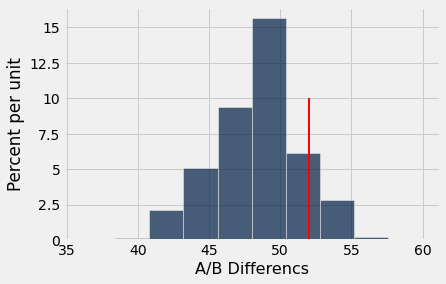
p_value = sum( yes_count >= 52) / reps
p_value
0.13446
Because the \(p\)-value is greater than 0.05, we fail to reject the null hypothesis. We have no evidence that Yes/No responses to the dating question depend on biological sex.
Dolphin study example
A group of 30 patients experiencing chronic depression were invited to a Caribean island to take part in therapy. The researchers randomly split the group in two. Half of them received clinical treatment for their depression only (along with a huge dose of beach therapy, one presumes). The other half received the same clinical treatment (and beach therapy) plus they went swimming with dolphins.
dolphin = Table.read_table('http://faculty.ung.edu/rsinn/dolphin.csv')
dolphin
| Treatment | Result |
|---|---|
| Dolphins | Improved |
| Dolphins | Improved |
| Dolphins | Improved |
| Dolphins | Improved |
| Dolphins | Improved |
| Dolphins | Improved |
| Dolphins | Improved |
| Dolphins | Improved |
| Dolphins | Improved |
| Dolphins | Improved |
... (20 rows omitted)
dolphin.pivot('Result','Treatment')
| Treatment | Did Not | Improved |
|---|---|---|
| Control | 12 | 3 |
| Dolphins | 5 | 10 |
The researchers want to know whether there is enough evidence to show that the dolphin therapy is significantly better than the clinical and beach therapy option. What null hypothesis will test their claim?
How could we test it? We can randomly assign the outcomes of Improved or Did Not to a simulated dolphin group. We then check to see how often 10 or more successes land in the randomized dolphin group. The sample method creates a table, so we finish with a column to produce the output as an array.
dolphin.sample(15, with_replacement = False).column(1)
array(['Did Not', 'Did Not', 'Improved', 'Did Not', 'Did Not', 'Did Not',
       'Improved', 'Improved', 'Did Not', 'Did Not', 'Did Not',
       'Improved', 'Did Not', 'Did Not', 'Improved'], dtype='<U8')
The following code block selects the simulated dolphin group and counts the number of participants in it who “Improved.”
sum( dolphin.sample(15, with_replacement = False).column(1) == 'Improved' )
6
improved_count = make_array()

# Set reps to 2,000 or less especially if working the cloud
reps = 25000

for i in range(reps):
    new_samp = dolphin.sample(15, with_replacement = False).column(1)
    new_count = sum(new_samp == 'Improved')
    improved_count = np.append(improved_count,new_count)

# Remove hashtag comment below to see the results array
# improved_count
ab_hist(improved_count,10)
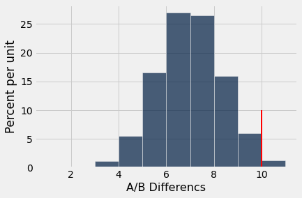
p_val = sum (improved_count >= 10) / reps
p_val
0.0126
The \(p\)-value is less than 0.05 which indicates the null hypothesis is unlikely to be true. Thus, we conclude the dolphin therapy appears to be beneficial to these patients, since a random distribution of the ‘Improved’ results would be unlikely to produce the observed pattern in the data.