26. Descriptive Statistics
from datascience import *
import numpy as np

%matplotlib inline

import matplotlib.pyplot as plots
plots.style.use('fivethirtyeight')

from scipy import stats
I keep some data frames in CSV format accessible from my website. One of them is called personality.csv and has, as you might imagine, personality variables. In this case, we are using the neuroanx subset which compares neuroticism, anxiety and several related variables:
- G21
Y/N response to “are you 21 years old or older?”
- SitClass
Front/middle/back response to “where do you prefer to sit in class?”
- Friends
Same/opposite/no difference response to “which sex do you find it easiest to make friends with.”
- TxRel
Toxic relationships beliefs, higher scores indicate more toxicity.
- Opt
Optimism, higher scores indicate more optimism
- SE
Self-esteem, higher score indicate higher levels of self-esteem
Standard descriptives for numeric variables
For each statistic below, we need an array of numeric data as the input. Let’s grab some data from the personality.csv file.
pers = Table.read_table('http://faculty.ung.edu/rsinn/neuroanx.csv')
pers.show(5)
| Sex | G21 | SitClass | Friends | TxRel | Anx | Opt | SE | Neuro |
|---|---|---|---|---|---|---|---|---|
| M | N | F | O | 26 | 23 | 20 | 70 | 10 |
| F | N | M | S | 21 | 24 | 22 | 68 | 11 |
| M | Y | F | E | 25 | 27 | 29 | 65 | 11 |
| M | Y | B | E | 22 | 30 | 28 | 61 | 15 |
| M | N | M | E | 23 | 40 | 26 | 64 | 16 |
... (137 rows omitted)
neuroanx = pers.select('Neuro','Anx')
neuro = neuroanx.column(0)
Mean ( \(\overline x\) )
Given an array, we simply use np.average or np.mean.
mean = np.mean(neuro)
mean
42.66197183098591
Sample size ( \(n\) )
n = len(neuro)
n
142
Standard deviation
A deviation is the distance between a data point and the mean. The sample standard deviation is the sum of the squared deviations divided by one less than the sample size (\(n-1\)).
devs_squared = ( neuro - mean ) ** 2
s = np.sqrt(sum(devs_squared / (n-1)))
s
13.946141246193354
We can test whether or not our formula is correct using the numpy function std with the ddof=1 option on. You will notice some rounding error.
np.std(neuro, ddof=1)
13.946141246193347
Print descriptives
The following three statistics are considered the standard descriptives by quantiative researchers. In a scientific report, each data set should be accompanied by these three descriptive statistics:
mean
sample size
standard deviation
To help detect skew and outliers, the median can be useful. Most researchers would not consider it a standard descriptive.
def describe (array):
mean = np.mean(array)
median = np.median(array)
n = len(array)
s = np.std(array, ddof=1)
print('The mean is', round(mean,2))
print('The median is', median)
print('The sample size is', n)
print('The standard deviation is', round(s,2))
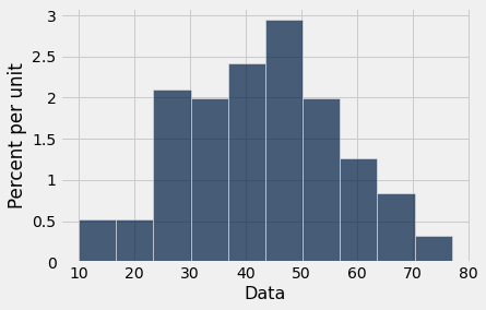
Table().with_column('Data',array).hist(0)
describe(neuro)
The mean is 42.66
The median is 43.0
The sample size is 142
The standard deviation is 13.95
Standardized scores
The formula for the standardized score is:
where \(x\) is the score from the data set and \(\mu\) and \(\sigma\) are the population mean and standard deviation respectively.
Creating a z_scores function
def z_scores(array):
    mean = np.mean(array)
    sd = np.std(array)
    return (array - mean) / sd
z_scores(neuro)
array([-2.35029814, -2.27833989, -2.27833989, -1.99050692, -1.91854867,
       -1.84659043, -1.77463219, -1.70267394, -1.48679921, -1.41484097,
       -1.34288272, -1.34288272, -1.34288272, -1.27092448, -1.27092448,
       -1.19896623, -1.19896623, -1.12700799, -1.05504975, -1.05504975,
       -1.05504975, -0.9830915 , -0.9830915 , -0.9830915 , -0.9830915 ,
       -0.9830915 , -0.9830915 , -0.91113326, -0.91113326, -0.91113326,
       -0.83917501, -0.83917501, -0.76721677, -0.76721677, -0.69525853,
       -0.69525853, -0.62330028, -0.62330028, -0.62330028, -0.62330028,
       -0.62330028, -0.62330028, -0.62330028, -0.62330028, -0.55134204,
       -0.55134204, -0.55134204, -0.47938379, -0.47938379, -0.40742555,
       -0.40742555, -0.40742555, -0.33546731, -0.33546731, -0.33546731,
       -0.26350906, -0.26350906, -0.19155082, -0.19155082, -0.19155082,
       -0.19155082, -0.19155082, -0.11959257, -0.11959257, -0.11959257,
       -0.11959257, -0.11959257, -0.11959257, -0.04763433,  0.02432391,
        0.02432391,  0.02432391,  0.09628216,  0.09628216,  0.09628216,
        0.09628216,  0.09628216,  0.09628216,  0.09628216,  0.1682404 ,
        0.1682404 ,  0.1682404 ,  0.24019865,  0.24019865,  0.24019865,
        0.24019865,  0.31215689,  0.31215689,  0.38411513,  0.38411513,
        0.38411513,  0.45607338,  0.45607338,  0.45607338,  0.45607338,
        0.52803162,  0.52803162,  0.52803162,  0.52803162,  0.52803162,
        0.59998987,  0.59998987,  0.67194811,  0.67194811,  0.67194811,
        0.74390635,  0.74390635,  0.74390635,  0.74390635,  0.74390635,
        0.74390635,  0.74390635,  0.8158646 ,  0.8158646 ,  0.8158646 ,
        0.8158646 ,  0.88782284,  0.95978108,  0.95978108,  1.03173933,
        1.03173933,  1.03173933,  1.03173933,  1.03173933,  1.03173933,
        1.10369757,  1.17565582,  1.17565582,  1.17565582,  1.39153055,
        1.46348879,  1.67936352,  1.67936352,  1.67936352,  1.67936352,
        1.75132177,  1.82328001,  1.89523826,  1.9671965 ,  2.18307123,
        2.18307123,  2.47090421])
Correlation
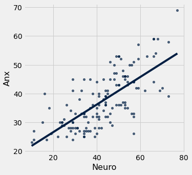
Let’s check to see if the two numeric variables of neuro (neuroticism) and anx (anxiety) are associated.
data = pers.select('Neuro','Anx')
data.show(5)
| Neuro | Anx |
|---|---|
| 10 | 23 |
| 11 | 24 |
| 11 | 27 |
| 15 | 30 |
| 16 | 40 |
... (137 rows omitted)
The correlation can be calculated in terms of \(z\)-scores (standardized scores).
meaning we multiply all \(xy\)-pairs of standardized scores, sum them and divide by \(n-1\).
The line of best fit always passes through the point
and has slope
where \(s_x\) and \(s_y\) are the sample standard deviations for the \(x\) and \(y\) variables respectively. In statistics, we write the line of best fit as
where \(a\) is the \(y\)-intercept and \(b\) is the slope.
Creating the reg_r and reg_stat function to calculate regression statistics and produce a scatter plot
def reg_r (tab):
    x = tab.column(0)
    y = tab.column(1)
    return sum(z_scores(x)*z_scores(y))/(n-1)
def reg_stat (tab):
    x = tab.column(0)
    y = tab.column(1)
    r = reg_r(tab)
    b = r * np.std(y) / np.std(x)
    a = np.mean(y) - b * np.mean(x)
    print('The correlation is ', r)
    print('The line of best fit is y =',round(a,4), '+',round(b,4),'x')
    tab.scatter(0,1, fit_line = True)
reg_stat(data)
The correlation is  0.7140323446533897
The line of best fit is y = 16.8451 + 0.4833 x
Creating the reg_shuffle function
While not a descriptive statistic, we do need a test for significant correlation. The idea is similar to A/B testing. We can randomly shuffle the \(y\)-variable and determine a distribution that assumes a zero correlation. We can compare our observed correlation to that value.
Let’s begin with the ab_shuffle function and tweak it slightly.
def ab_shuffle(tab):
    shuffle_group = tab.sample(with_replacement = False).column(0)
    shuffled_tab = tab.with_column("Shuffled Grouping",shuffle_group).select(2,1)
    return shuffled_tab
We want to feed our function a two-column table with the \(x\)-variable listed in the first column, and shuffle the second column. (The ab_shuffle function shuffles the first column.) We also need to return the original \(x\) column with the shuffled \(y\), e.g. the first and third columns.
def reg_shuffle(tab):
    shuffled_y = tab.sample(with_replacement = False).column(1)
    shuffled_tab = tab.with_column("Shuffled Y",shuffled_y).select(0,2)
    return shuffled_tab
reg_shuffle(neuroanx)
| Neuro | Shuffled Y |
|---|---|
| 10 | 37 |
| 11 | 34 |
| 11 | 28 |
| 15 | 26 |
| 16 | 44 |
| 17 | 24 |
| 18 | 32 |
| 19 | 32 |
| 22 | 23 |
| 23 | 40 |
... (132 rows omitted)
This will allow us to build a for loop and create the distribution of the test statistic that models a zero correlation.