24. Bootstrapping Tools¶

from datascience import *
import numpy as np

%matplotlib inline

import matplotlib.pyplot as plots
plots.style.use('fivethirtyeight')

from scipy import stats

Bootstrap Confidence Intervals¶

Steps in bootstrapping¶

	Step	Example
1.	Ask Question	What is the weight of babies born to smoking mothers?
2.	Get sample data	Get weights of 100 babies born to smokers
3.	Choose a statistic	Mean baby weight
4.	If population data available, calculate the statistic of the original sample	The mean weight of the 100 babies is 114 oz.
5.	Bootstrap the sample and calculate the statistic on the bootstrap sample	The mean weight of the 100 babies in bootstrap sample 1 is 115.3 oz.
6.	Repeat over many bootstrapped samples and record the results	Usually 1k samples is more than enough.
7.	Plot the distrubution and observe the uncertainty inherent from samples of a given size
8.	Find the 2.5 and 97.5 percentiles of the statistic over all of the bootstrap samples to compute a 95% confidence interval for the population parameter.

Creating `boot_one` function to generate a single bootstrap sample¶

The function below will resample from the first column of a table. Ensure your data table has a numeric variables in its first column.

def boot_one(table, samp_size):
    resample = table.sample(samp_size)
    return np.average(resample.column(0))

Let’s see how it works by loading sample data. Let’s resample the ‘Perfectionism’ variable.

pers = Table.read_table('http://faculty.ung.edu/rsinn/perfnarc.csv')
pers.show(5)

Sex	G21	Greek	AccDate	Stress1	Stress2	Perf	Narc
F	N	N	N	9	7	99	3
F	Y	N	Y	11	13	86	2
F	N	Y	N	15	14	118	4
F	N	N	Y	16	15	113	2
F	Y	N	Y	17	17	107	8

... (143 rows omitted)

We will feed the function a one-column table with the perfectionism scores. The function will resample (n = 25) and return the mean of that sample. Re-execute the code block several times to see what typical values in the distribution look like.

boot_one(pers.select('Perf'),25)

115.24

Step 1. Ask Question¶

What is the mean weight of babies born to smokers?

Step 2. Get Sample Data¶

Read in the Data. The data might be population data or sample data. Be aware of the diiference. If the data is population data, you will need to first create a sample from the population data, then resample it.

# This is sample data
births = Table.read_table('http://faculty.ung.edu/rsinn/baby.csv')
births.show(5)

Birth Weight	Gestational Days	Maternal Age	Maternal Height	Maternal Pregnancy Weight	Maternal Smoker
120	284	27	62	100	False
113	282	33	64	135	False
128	279	28	64	115	True
108	282	23	67	125	True
136	286	25	62	93	False

... (1169 rows omitted)

Step 3. Choose a statistic (mean)¶

The default statistic is the mean. If we want to estimate a different statistic like the median, then we would need to take the function boot_one and replace the np.average with np.median. In almost every case, especially in an introductory statistics course, we will estimate the mean.

Select the the birth weight of babies born to smokers as a one-column table of numeric values.

smoked = births.where('Maternal Smoker',True).select('Birth Weight')
smoked.show(5)

Birth Weight
128
108
143
144
141

... (454 rows omitted)

Step 4. Calculate the statistic of the original sample¶

Our original data is a sample, not a population, so every time we sample that sample we are resampling which is another name for bootstrapping.

Step 5. Bootstrap the sample and calculate the statistic on the bootstrap sample¶

Choose a resample size and sample with replacement.

boot_one(smoked,100)

113.46

Step 6. Repeat over many bootstrap samples¶

We use our standard for loop setup with a blank results array and np.append to add new results to it. Our resample size is 50, but we need 500 - 1,000 resamples for an accurate bootstrap distribution.

boot_samp = make_array()
resamp_size = 50

# Never need more than 1k reps, use 500 or fewer if working the cloud.
resample_reps = 1000

for i in range(resample_reps):
    new_boot = boot_one(smoked,resamp_size)
    boot_samp = np.append(boot_samp, new_boot)
    
# Remove the hashtag comment symbol to see the boot_samp results array
#boot_samp

def boot_hist (array):
    left = round(percentile(2.5, array),2)
    right = round(percentile(97.5, array),2)
    avg = round(np.average(array),2)
    tab = Table().with_column('Bootstrapped Sample',array)
    tab.hist(0)
    _ = plots.title('95% Confidence Interval')
    _ = plots.plot([left, left], [0, 0.1], color='red', lw=2)
    _ = plots.plot([right, right], [0, 0.1], color='red', lw=2)
    _ = plots.scatter(avg, 0, color="gold", s = 200,zorder=2);
    print("The 95% confidence interval lies between ", left," and ", right, ",")
    print("and the gold dot at x = ", avg, " is the mean of the bootstrapped sample distribution.")

boot_hist(boot_samp)

The 95% confidence interval lies between  108.3  and  118.88 ,
and the gold dot at x =  113.91  is the mean of the bootstrapped sample distribution.

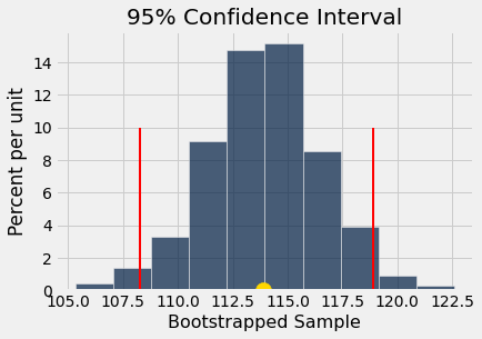
The 95% confidence interval endpoints are shown above the histogram: we are 95% confident that the true mean lies between 108.9 and 118.8.

Compare to resamples of size 200¶

Note that this resample size is 4 times larger than we used above. The law of large numbers indicates this larger (re)sample size should lead to a more accurate estimate.

boot_samp_2 = make_array()
resamp_size = 200

# Never need more than 1k reps, use 500 or fewer if working the cloud.
resample_reps = 1000

for i in range(resample_reps):
    new_boot = boot_one(smoked,resamp_size)
    boot_samp_2 = np.append(boot_samp_2, new_boot)
    
# Remove the hashtag comment symbol to see the boot_samp results array
#boot_samp

boot_hist(boot_samp_2)

The 95% confidence interval lies between  111.38  and  116.1 ,
and the gold dot at x =  113.86  is the mean of the bootstrapped sample distribution.

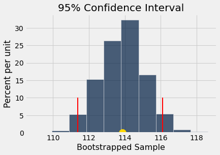
Compared to the confidence interval generated with a resample size of \(n=50\), the width of the new confidence interval is approximately 5 units less.

Intro to Applied Statistics