9. Functions and Subsetting using Chattahoochee National Forest Recreation Areas¶

from datascience import *
import numpy as np
from scipy.stats import t

%matplotlib inline
import matplotlib.pyplot as plots
plots.style.use('fivethirtyeight')

I keep some data frames in CSV format accessible from my website. One of them has recreation locations for the Chatahoochee National Forest.

chat = Table.read_table('http://faculty.ung.edu/rsinn/chattahoochee.csv')
chat.num_rows

chat

name	ranger station	type	county	lat deg	lat min	lat sec	lon deg	lon min	lon sec
PINHOTI #1, HWY 100	80301	TRAILHEAD	CHATTOOGA	34	23	21	-85	21	48
PINHOTI #1, HWY 136	80301	TRAILHEAD	WALKER	34	39	41	-85	3	30
JOHN'S MOUNTAIN OVERLOOK	80301	OBSERVATION SITE	WALKER	34	37	21	-85	5	51
KEOWN FALLS REC AREA	80301	PICNIC SITE	ALKER	34	36	33	-85	5	28
CHESTNUT MTN SHOOTING RANGE	80301	SHOOTING RANGE	WHITFIELD	34	37	14	-85	2	45
POCKET RECREATIONAL AREA	80301	CAMPGROUND	FLOYD	34	35	9	-85	4	57
HIDDEN CREEK REC. AREA	80301	CAMPGROUND	GORDON	34	30	52	-85	4	27
Cottonwood Patch Area	80307	CAMPGROUND	MURRAY	34	58	56	-84	38	20
SUMAC SHOOTING RANGE	80307	SHOOTING RANGE	GILMER	34	56	26	-84	42	35
HICKEY GAP	80307	CAMPGROUND	MURRAY	34	53	37	-84	40	18

... (122 rows omitted)

Exploring category data¶

`.group` Method¶

We have two obvious category variables: ‘county’ and ‘type’ of recreation area. While it looks numeric, the ‘ranger station’ ID number describes only handful of station.

Grouping by County¶

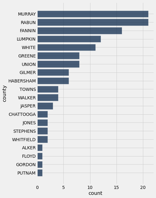
chat.group('county').sort('count',descending = True)

county	count
MURRAY	21
RABUN	21
FANNIN	16
LUMPKIN	12
WHITE	11
GREENE	8
UNION	8
GILMER	6
HABERSHAM	6
TOWNS	4

... (10 rows omitted)

chat.group('county').sort('count',descending = True).barh('county')

Recreation areas grouped by type¶

# Create a grouping table by type of recreation area.

# Create a bar chart showing for the grouping by type of recreation area sorted for most to least.

Recreation areas grouped by ranger station¶

# While the Ranger Station data may look numeric, it's not. 
# There are only a handful of them, so we can treat them like a category variables. 
# Create a grouping table by type of recreation area.

`.pivot` method¶

The best data display for two category variables is often a pivot table

chat.pivot('type','county').show()

C:\Users\robbs\anaconda3\envs\datasci\lib\site-packages\datascience\tables.py:920: VisibleDeprecationWarning: Creating an ndarray from ragged nested sequences (which is a list-or-tuple of lists-or-tuples-or ndarrays with different lengths or shapes) is deprecated. If you meant to do this, you must specify 'dtype=object' when creating the ndarray.
  values = np.array(tuple(values))

county	BOATING	CAMPGROUND	DAY USE	HORSE CAMP	INFORMATION	OBSERVATION SITE	PICNIC SITE	SHOOTING RANGE	TRAILHEAD
ALKER	0	0	0	0	0	0	1	0	0
CHATTOOGA	0	0	0	0	0	0	0	0	2
FANNIN	2	5	0	0	0	0	0	0	9
FLOYD	0	1	0	0	0	0	0	0	0
GILMER	0	0	0	0	0	1	1	1	3
GORDON	0	1	0	0	0	0	0	0	0
GREENE	3	1	0	0	0	0	0	1	3
HABERSHAM	1	2	0	0	1	0	2	0	0
JASPER	0	0	2	0	0	0	0	0	1
JONES	0	0	0	0	0	0	2	0	0
LUMPKIN	0	5	1	0	0	1	1	0	4
MURRAY	0	6	2	0	0	2	1	0	10
PUTNAM	0	1	0	0	0	0	0	0	0
RABUN	0	8	1	1	0	1	2	1	7
STEPHENS	0	0	0	0	0	0	0	0	2
TOWNS	0	2	0	0	1	0	0	0	1
UNION	0	3	0	0	0	0	0	0	5
WALKER	0	0	1	0	0	1	0	0	2
WHITE	0	3	1	0	2	0	1	0	4
WHITFIELD	0	0	0	0	0	0	0	1	1

Suppose Mina and Jo were interested in hiking and picnic areas. Recall that grouping tables and pivot tables are still tables, so table methods can be used on them. We can select three columns of the pivot table and sort by number of picnic sites.

chat.pivot('type','county').select('county','PICNIC SITE','TRAILHEAD')

county	PICNIC SITE	TRAILHEAD
ALKER	1	0
CHATTOOGA	0	2
FANNIN	0	9
FLOYD	0	0
GILMER	1	3
GORDON	0	0
GREENE	0	3
HABERSHAM	2	0
JASPER	0	1
JONES	2	0

... (10 rows omitted)

We can use parentheses to allow a “text wrapping” effect so we can add returns and indents for clarity when using multiple methods.

(chat.pivot('type','county')
     .select('county','PICNIC SITE','TRAILHEAD')
     .sort('PICNIC SITE', descending = True))

county	PICNIC SITE	TRAILHEAD
HABERSHAM	2	0
JONES	2	0
RABUN	2	7
ALKER	1	0
GILMER	1	3
LUMPKIN	1	4
MURRAY	1	10
WHITE	1	4
CHATTOOGA	0	2
FANNIN	0	9

... (10 rows omitted)

If we sort twice, we can find which of the counties with the most picnic areas have the most trailheads. Notice how the two sorts are run by priority.

(chat.pivot('type','county')
     .select('county','PICNIC SITE','TRAILHEAD')
     .sort('TRAILHEAD', descending = True)
     .sort('PICNIC SITE', descending = True))

county	PICNIC SITE	TRAILHEAD
RABUN	2	7
HABERSHAM	2	0
JONES	2	0
MURRAY	1	10
LUMPKIN	1	4
WHITE	1	4
GILMER	1	3
ALKER	1	0
FANNIN	0	9
UNION	0	5

... (10 rows omitted)

Cleaning Data¶

The latitude and longitude columns are in deg-min-sec format rather than decimal format. We can use several approaches to create arrays of latitude and longitude in decimal form:

The .column method used six times with formula implemented manually
A user-defined function using .apply method (still need .column method)
A user-defined function using full power of the .apply method

1. The `.column` method¶

We take the 3 latitude columns and perform the arithmetic ourselves.

latd = chat.column('lat deg')
latm = chat.column('lat min')
lats = chat.column('lat sec')

lat = latd + latm / 60 + lats / 3600

chat_lat = chat.with_column('lat', lat).drop('lat deg','lat min','lat sec')

#Complete the work by doing the same steps for longitude

# Create a table called chat_lat_lon that contains two columns "lat" and "lon" which have
# the decimal values for latitude and longitude.

chat_lat_lon = ...

2. User-defined functions¶

def dms_to_dec(d,m,s):
    return d + m / 60 + s / 3600

# Use the function defined above to create two arrays, one for latitudes and one for longitudes 

3. User-defined function with `.apply` method¶

The .apply method, if a column is not specified, just works row by row. For this reason, we do not have to use the .column method first. We can just feed the function a table with the proper three columns.

def deg_2_dec(my_row):
    d = my_row.item(0)
    m = my_row.item(1)
    s = my_row.item(2)
    return d + m/60 + s/3600

lat = chat.select('lat deg','lat min','lat sec').apply(deg_2_dec)
lat

array([34.38916667, 34.66138889, 34.6225    , 34.60916667, 34.62055556,
       34.58583333, 34.51444444, 34.98222222, 34.94055556, 34.89361111,
       34.82611111, 34.73388889, 34.86277778, 34.83472222, 34.82027778,
       34.82027778, 34.81472222, 34.81      , 34.78611111, 34.93861111,
       34.89888889, 33.15444444, 34.78861111, 33.11944444, 34.9425    ,
       34.95027778, 33.73194444, 34.86222222, 33.72083333, 33.64666667,
       33.56805556, 33.55      , 33.20833333, 34.84555556, 34.88361111,
       34.86888889, 34.7925    , 34.74      , 34.7025    , 34.76388889,
       34.76555556, 34.74194444, 34.70555556, 34.67861111, 34.89638889,
       34.72138889, 34.695     , 34.68      , 34.665     , 34.62888889,
       34.60777778, 34.59666667, 34.58388889, 34.67416667, 34.87611111,
       34.95472222, 34.75194444, 34.81555556, 34.83694444, 34.92333333,
       34.68138889, 33.6475    , 33.24222222, 33.17972222, 34.91972222,
       34.94777778, 34.90027778, 34.88138889, 34.95555556, 34.92833333,
       34.82055556, 34.76111111, 34.7575    , 34.785     , 34.78388889,
       34.83222222, 34.8275    , 34.84694444, 34.91138889, 34.875     ,
       34.96111111, 34.95444444, 34.9275    , 34.69861111, 34.58555556,
       34.55888889, 34.505     , 34.4925    , 34.50138889, 34.49527778,
       34.50222222, 34.63722222, 34.76      , 34.77777778, 34.79      ,
       34.75111111, 34.70194444, 34.72416667, 34.68888889, 34.75888889,
       34.615     , 34.57888889, 34.63861111, 34.98833333, 34.99083333,
       34.93388889, 34.92583333, 34.88194444, 34.8725    , 34.87277778,
       34.87027778, 34.85416667, 34.8525    , 34.85527778, 34.85416667,
       34.85388889, 34.74111111, 34.85722222, 34.75666667, 34.63888889,
       34.58861111, 34.81666667, 34.73916667, 33.20777778, 33.64916667,
       33.66361111, 34.94472222, 34.93083333, 34.815     , 34.75944444,
       34.7975    , 34.71      ])

lon = chat.select('lon deg','lon min','lon sec').apply(deg_2_dec)
lon

array([-84.63666667, -84.94166667, -84.9025    , -84.90888889,
       -84.95416667, -84.9175    , -84.92583333, -83.36111111,
       -83.29027778, -83.32833333, -83.41805556, -83.30944444,
       -83.48305556, -83.30361111, -83.44805556, -83.43388889,
       -83.43888889, -83.36083333, -83.37277778, -83.33972222,
       -83.35444444, -82.40222222, -84.87055556, -82.49861111,
       -83.3325    , -83.39527778, -82.70944444, -83.34305556,
       -82.70861111, -82.71      , -82.72777778, -82.69972222,
       -82.60472222, -83.71027778, -83.73222222, -83.75583333,
       -83.76111111, -83.85972222, -83.85055556, -83.92694444,
       -83.93416667, -82.07777778, -82.08222222, -82.00055556,
       -82.09222222, -83.86694444, -83.78972222, -83.99888889,
       -82.0825    , -83.86583333, -83.845     , -83.95472222,
       -83.81555556, -82.02472222, -82.18916667, -82.22055556,
       -82.10361111, -83.69916667, -83.72083333, -83.90583333,
       -82.06166667, -82.85305556, -82.18638889, -82.18277778,
       -82.83111111, -82.79861111, -82.7775    , -82.64666667,
       -82.66472222, -82.73583333, -82.55694444, -82.52916667,
       -82.52333333, -82.44666667, -82.44555556, -82.37388889,
       -82.38111111, -82.40305556, -82.38194444, -82.425     ,
       -82.4425    , -82.4475    , -82.45527778, -82.57916667,
       -82.60027778, -82.54527778, -82.61833333, -82.49916667,
       -82.51833333, -82.51      , -82.49333333, -82.28055556,
       -82.28833333, -82.26333333, -82.21611111, -82.21666667,
       -82.21083333, -82.16166667, -82.10833333, -82.2175    ,
       -84.92722222, -84.87055556, -84.91694444, -83.36666667,
       -83.41166667, -83.48305556, -83.32194444, -83.43388889,
       -83.43444444, -83.34888889, -83.46      , -83.42027778,
       -83.385     , -83.34111111, -83.35055556, -83.34611111,
       -83.32888889, -83.35027778, -83.935     , -83.80583333,
       -83.86027778, -82.27222222, -82.02972222, -82.17944444,
       -82.86694444, -82.63      , -82.80444444, -82.45472222,
       -82.69083333, -82.25111111, -82.21555556, -82.21027778])

chattahoochee = (chat.select('name','type','county')
                 .with_columns(
                     'lat',lat,
                     'lon',lon))
chattahoochee

name	type	county	lat	lon
PINHOTI #1, HWY 100	TRAILHEAD	CHATTOOGA	34.3892	-84.6367
PINHOTI #1, HWY 136	TRAILHEAD	WALKER	34.6614	-84.9417
JOHN'S MOUNTAIN OVERLOOK	OBSERVATION SITE	WALKER	34.6225	-84.9025
KEOWN FALLS REC AREA	PICNIC SITE	ALKER	34.6092	-84.9089
CHESTNUT MTN SHOOTING RANGE	SHOOTING RANGE	WHITFIELD	34.6206	-84.9542
POCKET RECREATIONAL AREA	CAMPGROUND	FLOYD	34.5858	-84.9175
HIDDEN CREEK REC. AREA	CAMPGROUND	GORDON	34.5144	-84.9258
Cottonwood Patch Area	CAMPGROUND	MURRAY	34.9822	-83.3611
SUMAC SHOOTING RANGE	SHOOTING RANGE	GILMER	34.9406	-83.2903
HICKEY GAP	CAMPGROUND	MURRAY	34.8936	-83.3283

... (122 rows omitted)

Maps using lat-lon coordinates¶

Marker.map_table(chattahoochee.select('lat','lon','name'))

Make this Notebook Trusted to load map: File -> Trust Notebook

Circle.map_table(chattahoochee.select('lat','lon','name'))

Make this Notebook Trusted to load map: File -> Trust Notebook

Recreation areas near Dahlonega¶

Miles per degree of latitude¶

The distance between latitude lines are consistent, or would be if the earth were a sphere. Taking the radius of a spherical earth as 4,000 miles, we can chop the circumference of the earth into 360 equally sized pieces, one for each of the \(360^\circ\), using the formula for the circumference of circule based on its radius.

\[C = 2\pi r \approx 25133 \text{ mi}\]

The distance between latitude lines that are one degree apart is approximately 70 miles which a bit of basic geometry will demonstrate.

r = 4000
circumference = 2 * np.pi * r
circumference

25132.741228718343

mile_per_degree_lat = circumference / 360 
mile_per_degree_lat

69.81317007977317

This is why we round to 70 miles per degree of latitude to make life simpler.

Miles per degree of longitude¶

The distance between lines of longitude varies from a maximum at the equator to near-zero at the north or south pole. Within a hudred yards of the north pole, the distance between degrees of longitude would be one or two footsteps. At the equator, assuming the eath is spherical, the distance would the same as for latitude, or about 70 miles.

We can find the radius around the earth at \(34.5^\circ\) latitude, a good approximation based on UNG’s Dahlonega campus coordinates:

\[(34.5279^\circ N, 83.9844^\circ W)\]

If we call \(x\) the new radius, the one specific to the latitude, then:

\[\cos L = \frac{x}{r}\]

where

\[\begin{split}\begin{align*} L &= \text{ degrees latitude} \\ R &= \text{ radius} \end{align*}\end{split}\]

The numpy package expects radians, not degrees, so the value for \(x\) will be as follows.

x = np.cos(34.5 * np.pi / 180) * r
x

3296.5047544880626

With the new radius \(x\), we do the same as before. Determine the circumference and divide it by 360.

x_circumference = 2 * np.pi * x
x_circumference

20712.550238447046

mile_per_degree_long = x_circumference / 360
mile_per_degree_long

57.534861773464016

This means that near Dahlonega, GA, there about 70 miles between each degree of latitude and about 57.5 miles between each degree of longitude. Suppose that we want to find all the recreation areas that are within 30 miles east or west of the UNG Dahlonega campus and within 30 miles north and south.

lat_adj = 30/70
round(lat_adj,2)

0.43

lon_adj = 30 / 57.5
round(lon_adj,2)

0.52

chat_near_dahlonega = (chattahoochee.where('lat',are.between(34.5 - lat_adj,34.5+lat_adj))
                       .where('lon',are.between(-84 - lon_adj, -84+lon_adj)))
chat_near_dahlonega

name	type	county	lat	lon
JACK'S RIVER FIELDS CAMPGROUND	CAMPGROUND	FANNIN	34.8628	-83.4831
LAKE BLUE RIDGE CG	CAMPGROUND	FANNIN	34.8456	-83.7103
LAKEWOOD LANDING	BOATING	FANNIN	34.8836	-83.7322
MORGANTON PT. REC. AREA	CAMPGROUND	FANNIN	34.8689	-83.7558
TOCCOA SANDY BOTTOMS	BOATING	FANNIN	34.7925	-83.7611
DEEP HOLE REC. AREA	CAMPGROUND	FANNIN	34.74	-83.8597
FRANK GOSS REC. AREA	CAMPGROUND	FANNIN	34.7025	-83.8506
MULKY REC. AREA	CAMPGROUND	UNION	34.7639	-83.9269
COOPER CREEK REC. AREA	CAMPGROUND	UNION	34.7656	-83.9342
ROCK CR. DISPERSED SITE	CAMPGROUND	MURRAY	34.7214	-83.8669

... (12 rows omitted)

Circle.map_table(chat_near_dahlonega.select('lat','lon','name'))

Make this Notebook Trusted to load map: File -> Trust Notebook

# Create a map of all recreation areas in White County.

# Create a map of all trailheads in Rabun County.

Using predicates in `.where` methods¶

What if we want to find all recreation areas within nearby counties? The basic .where method only allows us to filter based on one county name at a time, but what if we use the predicate are.contained_in? Life becomes much easier.

Task: create a map of all recreation areas in Lumkin and White counties.¶

Lumpkin_White = chattahoochee.where('county', are.contained_in ('LUMPKIN WHITE'))

Lumpkin_White.show()

name	type	county	lat	lon
DESOTO FALLS REC. AREA	CAMPGROUND	LUMPKIN	34.7056	-82.0822
WOODY GAP REC. AREA	PICNIC SITE	LUMPKIN	34.6786	-82.0006
CHESTATEE OVERLOOK	OBSERVATION SITE	LUMPKIN	34.68	-83.9989
WATERS CREEK REC. AREA	CAMPGROUND	LUMPKIN	34.665	-82.0825
MONTGOMERY CREEK	DAY USE	LUMPKIN	34.6289	-83.8658
JONES CR. DISPERSED AREA	TRAILHEAD	LUMPKIN	34.6078	-83.845
WHISSENHUNT ORV AREA	TRAILHEAD	LUMPKIN	34.5967	-83.9547
NIMBERWILL DISPERSED AREA	TRAILHEAD	LUMPKIN	34.5839	-83.8156
DOCKERY LAKE REC. AREA	CAMPGROUND	LUMPKIN	34.6742	-82.0247
DICKS CREEK USE AREA (04)	CAMPGROUND	LUMPKIN	34.6814	-82.0617
MOUNT YONAH TRAILHEAD	TRAILHEAD	WHITE	34.6372	-82.2806
ANNA RUBY FALLS REC AREA	INFORMATION	WHITE	34.76	-82.2883
ANDREWS COVE REC. AREA	CAMPGROUND	WHITE	34.7778	-82.2633
UPPER CHATT. RIVER CAMPGROUND	CAMPGROUND	WHITE	34.79	-82.2161
LOW GAP CAMPGROUND	CAMPGROUND	WHITE	34.7511	-82.2167
DUKES CREEK REC AREA	PICNIC SITE	WHITE	34.7019	-82.2108
HOG PEN GAP	TRAILHEAD	WHITE	34.7242	-82.1617
BOGGS CR. REC. AREA	CAMPGROUND	LUMPKIN	34.6889	-82.1083
JASUS CREEK	DAY USE	WHITE	34.7589	-82.2175
JAKE--BULL MTN. COMPLEX	TRAILHEAD	LUMPKIN	34.5886	-83.8603
SCENIC BY-WAY PULL OFF	INFORMATION	WHITE	34.7594	-82.2511
HORSE TROUGH FALL	TRAILHEAD	WHITE	34.7975	-82.2156
RAVEN CLIFFS	TRAILHEAD	WHITE	34.71	-82.2103

Circle.map_table(Lumpkin_White.select('lat','lon','name'))

Make this Notebook Trusted to load map: File -> Trust Notebook

chat.where(truth_array)

---------------------------------------------------------------------------
NameError                                 Traceback (most recent call last)
<ipython-input-40-0883367b720f> in <module>
----> 1 chat.where(truth_array)

NameError: name 'truth_array' is not defined

# Create a map of all Chattahoochee trailheads in Lumpkin, White, Rabun and Union counties.

Intro to Applied Statistics

9. Functions and Subsetting using Chattahoochee National Forest Recreation Areas¶

Exploring category data¶

.group Method¶

Grouping by County¶

Recreation areas grouped by type¶

Recreation areas grouped by ranger station¶

.pivot method¶

Cleaning Data¶

1. The .column method¶

2. User-defined functions¶

3. User-defined function with .apply method¶

Maps using lat-lon coordinates¶

Recreation areas near Dahlonega¶

Miles per degree of latitude¶

Miles per degree of longitude¶

Using predicates in .where methods¶

Task: create a map of all recreation areas in Lumkin and White counties.¶

`.group` Method¶

`.pivot` method¶

1. The `.column` method¶

3. User-defined function with `.apply` method¶

Using predicates in `.where` methods¶