Sampling the Hypergeometric Distribution

We will use the deck of cards data frame that was shown in the appendix.

Show code cell source Hide code cell source

values <- rep(2:14,4)
suits <- c(rep('S',13), rep('H',13), rep('D',13), rep('C',13))
deck_df <- data.frame(v = values, suits = factor(suits))
head(deck_df,5)

v	suits
2	S
3	S
4	S
5	S
6	S

As was shown at the link above, we can draw a hand and account only for the suits of the cards drawn using the function sample(). To illustrate below, we will draw five cards at random from a standard deck of playing cards and store them in the variable hand. We will also show how to count the number of spades that are in the hand.

hand <- sample(deck_df$suits, 5)
cat('In this hand, the number of\n   spades = ', sum( hand  == 'S' ))
hand

In this hand, the number of
   spades =  2

1. S
2. S
3. C
4. D
5. C

Levels:

1. 'C'
2. 'D'
3. 'H'
4. 'S'

Example: Number of Spades Drawn into a Spades Hand

Spades are the permanent trump suit in the game of Spades. In a game of Spades with four players, each player is dealt a 13-card hand. Let’s deal a hand and count the number of spades in it.

hand <- sample(deck_df$suits, 13)
cat('In this hand, the number of\n   spades = ', sum( hand  == 'S' ))

In this hand, the number of
   spades =  3

The CLT and Law of Large Numbers

Our sample size is fixed at \(k=13\) for drawing a spades hand. Thus, the CLT will have no room to improve the estimate. However, using the Law of Large numbers, we can draw thousands (or millions) of hands.

Expected Value of the Hypergeometric Distribution

In a collection of \(N\) objects \(K\) of which are considered successes, the probability of \(k\) successful draws out of \(n\) total draws is given by hypergeometric distribution, we have the following pdf:

\[P(k) = \frac{\binom{K}{k}\binom{N-K}{n-k}}{\binom{N}{n}}\]

The expected value of this distribution is given by:

\[E(X) = n\frac{K}{N}\]

Theoretical Expected Value for our Example

For the card game Spades, \(N=52, K=13, n = 13\) and \(k\) varies between 0 and 13 inclusive. Thus, for Spades:

\[E(X) = 13\left(\frac{13}{52}\right) = \frac{13}{4} = 3.25\]

This table summarizes the investigation to include five examples from the sampling distribution of Drawing a Spades hand:

Hands Drawn	N	K	E(X)	Simulation Grand Mean
1,000	52	13	3.25
2,000	52	13	3.25	3.2325
5,000	52	13	3.25	3.2394
10,000	52	13	3.25	3.2527
50,000	52	13	3.25	3.24732
100,000	52	13	3.25	3.23414

Distribution for Number of Spades in a Hand

Using the for loop created the previous section of these notes, we can copy-paste and tweak as needed.

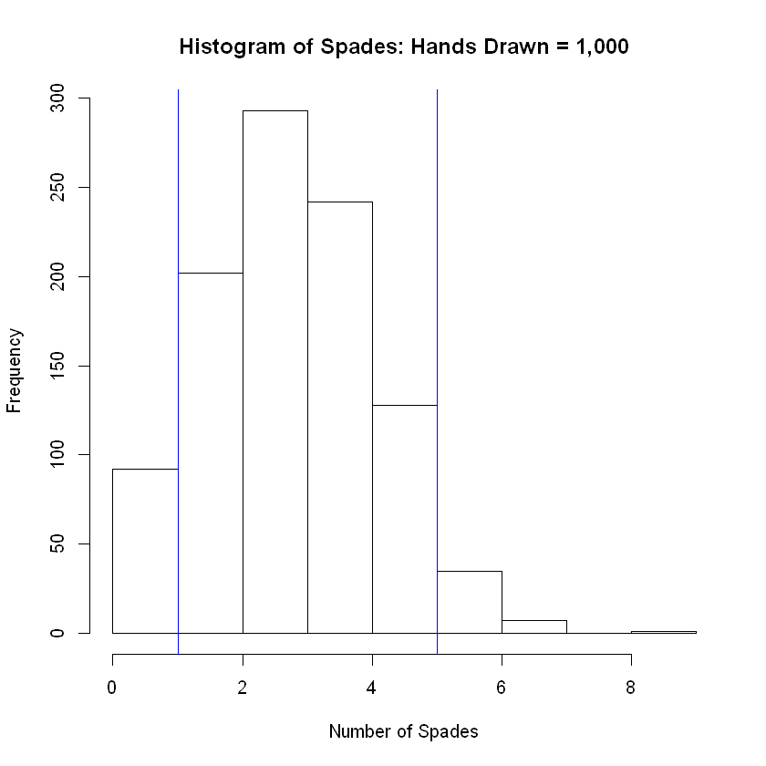
num_success <- c()     # create a vector to store the number of successes for each sample drawn
num_samps = 1000       # set the number of samples to be drawn

for (i in 1:num_samps){
    hand <- sample(deck_df$suits, 13)     # draw 13 cards, count number of Spades
    num_success[i] <- sum( hand  == 'S' )     # count and store the number of Spades from this trial
}

lower <- quantile(num_success, prob = 0.05)     # Calcuate the 5th percentile.
upper <- quantile(num_success, prob = 0.95)     # Calcuate the 95th percentile.
cat('The grand mean of the simulated distribution is equal to\n   ',mean(num_success) )
hist(num_success, breaks = 8, main = 'Histogram of Spades: Hands Drawn = 1,000', xlab = 'Number of Spades')
abline( v = lower, col="blue")     # Add vertical line at 5th percentile
abline(v = upper, col="blue")      # Add vertical line at 95th percentile 

The grand mean of the simulated distribution is equal to
    3.24

Collecting the Results

I will create a table here that gathers the results from sampling distribution with sample size 13 (fixed by problem scenario) and with increasing number of samples drawn.

Hands Drawn	E(X)	Simulation Grand Mean
1,000	3.25	3.252
2,000	3.25	3.2325
5,000	3.25	3.2394
10,000	3.25	3.2527
50,000	3.25	3.24732
100,000	3.25	3.23414

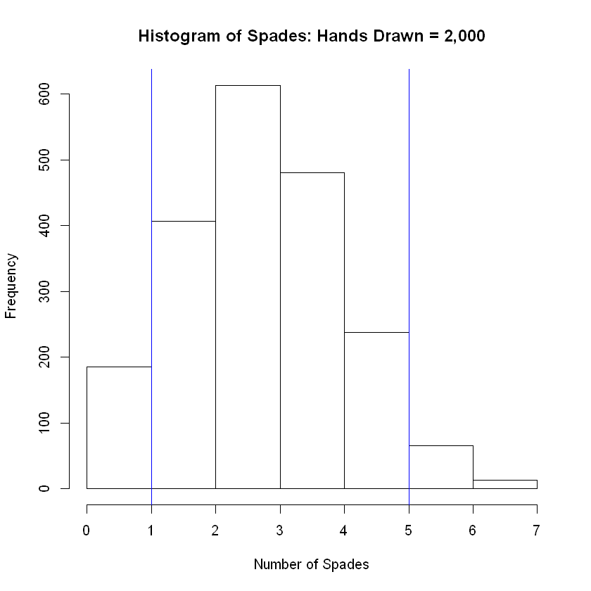
num_success <- c()     # create a vector to store the number of successes for each sample drawn
num_samps = 2000       # set the number of samples to be drawn

for (i in 1:num_samps){
    hand <- sample(deck_df$suits, 13)     # draw 13 cards, count number of Spades
    num_success[i] <- sum( hand  == 'S' )     # count and store the number of Spades from this trial
}

lower <- quantile(num_success, prob = 0.05)     # Calcuate the 5th percentile.
upper <- quantile(num_success, prob = 0.95)     # Calcuate the 95th percentile.
cat('The grand mean of the simulated distribution is equal to\n   ',mean(num_success) )
hist(num_success, breaks = 8, main = 'Histogram of Spades: Hands Drawn = 2,000', xlab = 'Number of Spades')
abline( v = lower, col="blue")     # Add vertical line at 5th percentile
abline(v = upper, col="blue")      # Add vertical line at 95th percentile 

The grand mean of the simulated distribution is equal to
    3.2025

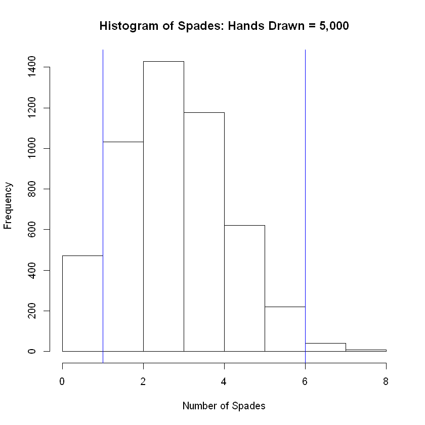
num_success <- c()     # create a vector to store the number of successes for each sample drawn
num_samps = 5000       # set the number of samples to be drawn

for (i in 1:num_samps){
    hand <- sample(deck_df$suits, 13)     # draw 13 cards, count number of Spades
    num_success[i] <- sum( hand  == 'S' )     # count and store the number of Spades from this trial
}

lower <- quantile(num_success, prob = 0.05)     # Calcuate the 5th percentile.
upper <- quantile(num_success, prob = 0.95)     # Calcuate the 95th percentile.
cat('The grand mean of the simulated distribution is equal to\n   ',mean(num_success) )
hist(num_success, breaks = 8, main = 'Histogram of Spades: Hands Drawn = 5,000', xlab = 'Number of Spades')
abline( v = lower, col="blue")     # Add vertical line at 5th percentile
abline(v = upper, col="blue")      # Add vertical line at 95th percentile 

The grand mean of the simulated distribution is equal to
    3.2492

num_success <- c()     # create a vector to store the number of successes for each sample drawn
num_samps = 10000       # set the number of samples to be drawn

for (i in 1:num_samps){
    hand <- sample(deck_df$suits, 13)     # draw 13 cards, count number of Spades
    num_success[i] <- sum( hand  == 'S' )     # count and store the number of Spades from this trial
}

lower <- quantile(num_success, prob = 0.05)     # Calcuate the 5th percentile.
upper <- quantile(num_success, prob = 0.95)     # Calcuate the 95th percentile.
cat('The grand mean of the simulated distribution is equal to\n   ',mean(num_success) )
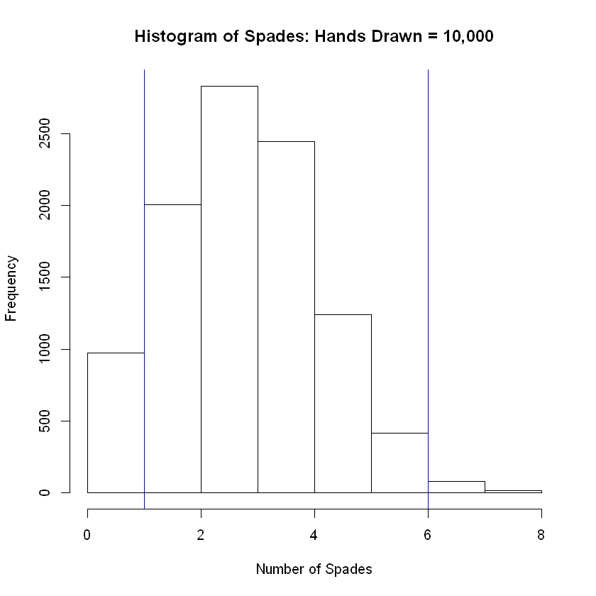
hist(num_success, breaks = 8, main = 'Histogram of Spades: Hands Drawn = 10,000', xlab = 'Number of Spades')
abline( v = lower, col="blue")     # Add vertical line at 5th percentile
abline(v = upper, col="blue")      # Add vertical line at 95th percentile 

The grand mean of the simulated distribution is equal to
    3.2474

num_success <- c()     # create a vector to store the number of successes for each sample drawn
num_samps = 50000       # set the number of samples to be drawn

for (i in 1:num_samps){
    hand <- sample(deck_df$suits, 13)     # draw 13 cards, count number of Spades
    num_success[i] <- sum( hand  == 'S' )     # count and store the number of Spades from this trial
}

lower <- quantile(num_success, prob = 0.05)     # Calcuate the 5th percentile.
upper <- quantile(num_success, prob = 0.95)     # Calcuate the 95th percentile.
cat('The grand mean of the simulated distribution is equal to\n   ',mean(num_success) )
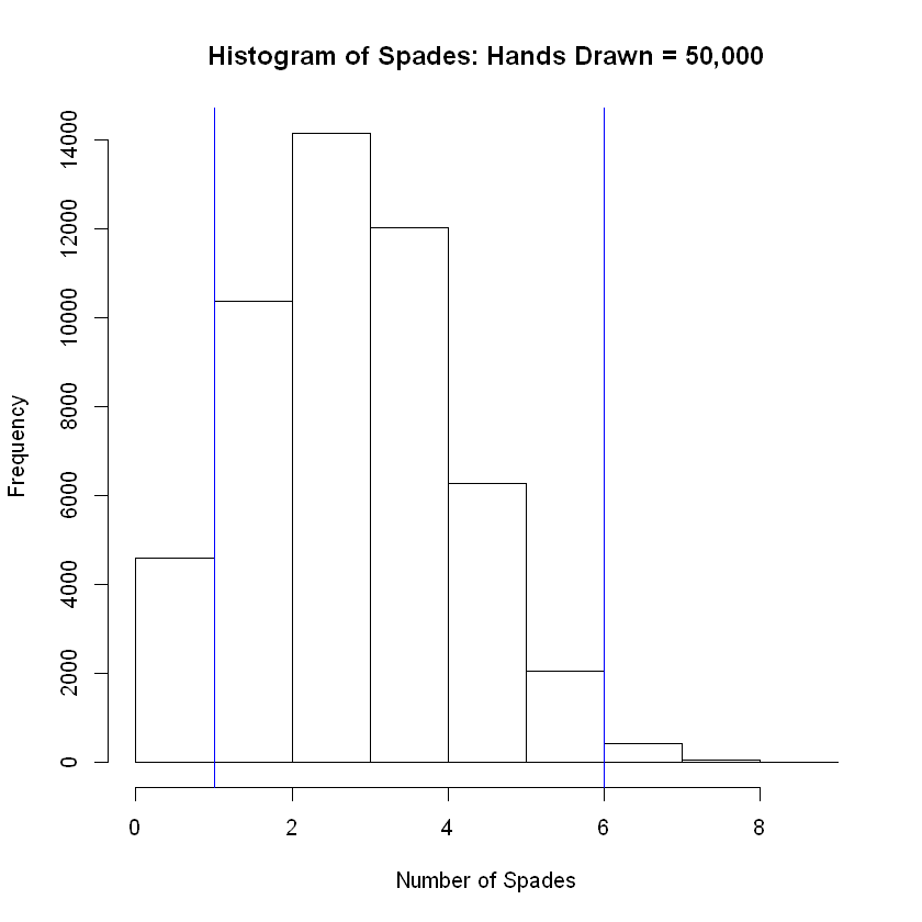
hist(num_success, breaks = 12, main = 'Histogram of Spades: Hands Drawn = 50,000', xlab = 'Number of Spades')
abline( v = lower, col="blue")     # Add vertical line at 5th percentile
abline(v = upper, col="blue")      # Add vertical line at 95th percentile 

The grand mean of the simulated distribution is equal to
    3.25164

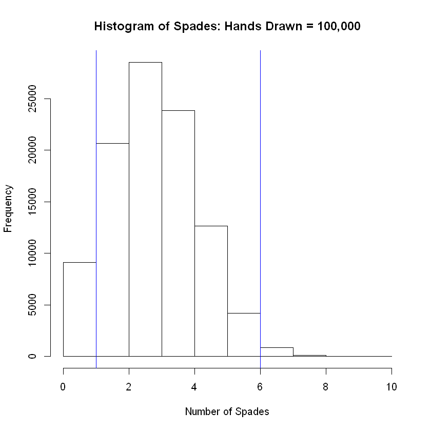
num_success <- c()     # create a vector to store the number of successes for each sample drawn
num_samps = 100000     # set the number of samples to be drawn

for (i in 1:num_samps){
    hand <- sample(deck_df$suits, 13)     # draw 13 cards, count number of Spades
    num_success[i] <- sum( hand  == 'S' )     # count and store the number of Spades from this trial
}

lower <- quantile(num_success, prob = 0.05)     # Calcuate the 5th percentile.
upper <- quantile(num_success, prob = 0.95)     # Calcuate the 95th percentile.
cat('The grand mean of the simulated distribution is equal to\n   ',mean(num_success) )
hist(num_success, breaks = 12, main = 'Histogram of Spades: Hands Drawn = 100,000', xlab = 'Number of Spades')
abline( v = lower, col="blue")     # Add vertical line at 5th percentile
abline(v = upper, col="blue")      # Add vertical line at 95th percentile 

The grand mean of the simulated distribution is equal to
    3.25672