Sampling with Negative Binomial Distribution

Recall the following details of the Negative Binomial Distribution pdf:

Given the following values:

• \(n\) indicates the number of trials.

• \(k\) indicates the number of successes needed for overall success.

• \(p\) indicates the probability of success.

• \(q=1-p\) indicates the probability of failure.

• \(X\) represents the number of the last well drilled to achieve overall success.

The closed form pdf for a negative binomial distribution is as follows:

\[P(X=x) = \binom{n-1}{k-1}p^kq^{n-k}\]

The rflip() Function

We need to be able to use rflip() inside our while loop.

Show code cell source Hide code cell source

rflip <- function(n=1, prob=.5, quiet=FALSE, verbose = !quiet, summarize = FALSE, 
                  summarise = summarize) {
	if ( ( prob > 1 && is.integer(prob) ) ) {  
		# swap n and prob
		temp <- prob
		prob <- n
		n <- temp
	}
	if (summarise) {
	  heads <- rbinom(1, n, prob)
	  return(data.frame(n = n, heads = heads, tails = n - heads, prob = prob))
	} else {
	  r <- rbinom(n,1,prob)
	  result <- c('T','H')[ 1 + r ]
	  heads <- sum(r)
	  attr(heads,"n") <- n
	  attr(heads,"prob") <- prob 
	  attr(heads,"sequence") <- result
	  attr(heads,"verbose") <- verbose
	  class(heads) <- 'cointoss'
	  return(heads)
	}
}

The expected value is given below:

\[E(X) = \frac{k}{p}\]

Oil fields: 25% chance of successes

\[E(X) = \frac{3}{\frac{1}{4}} = 12\]

k <- 0     # Initialize number of successes index
n <- 0     # Initialize number of total trials needed for success to occur
while (k < 3 && n < 20) {
   k <- k + rflip(1, prob = 1/4, summarize = TRUE)[1,2]
   n <- n + 1
}
n

11

Now we can run the for loop with \(k=100\).

num_trials_needed <- c()     # create a vector to store the number of trials needed in while loop
num_samps = 100              # set the number of times to run the simulation

for (i in 1:num_samps){
    k <- 0     # Initialize number of successes index
    n <- 0     # Initialize number of total trials needed for success to occur
    while (k < 3 && n < 20) {
        k <- k + rflip(1, prob = 1/4, summarize = TRUE)[1,2]
        n <- n + 1
    }
    num_trials_needed[i] <- n     # store the number of trials need in this simulation
}

lower <- quantile(num_trials_needed, prob = 0.05)     # Calcuate the 5th percentile.
upper <- quantile(num_trials_needed, prob = 0.95)     # Calcuate the 95th percentile.
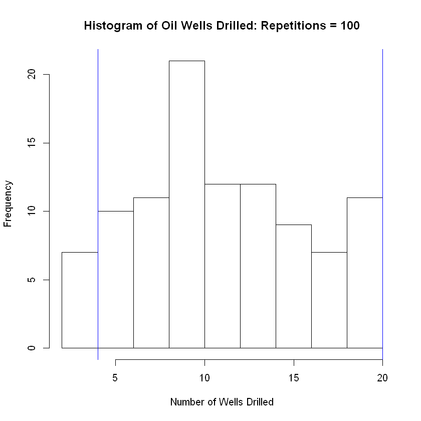
cat('The grand mean of the number of trials needed to achieve success is equal to\n   ',mean(num_trials_needed) )
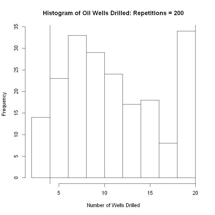
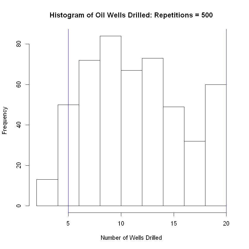
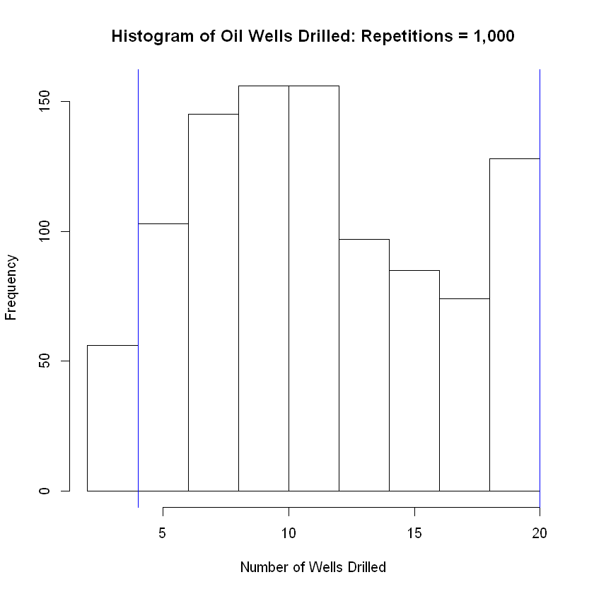
hist(num_trials_needed, breaks = 8, main = 'Histogram of Oil Wells Drilled: Repetitions = 100', xlab = 'Number of Wells Drilled')
abline( v = lower, col="blue")     # Add vertical line at 5th percentile
abline(v = upper, col="blue")      # Add vertical line at 95th percentile 

The grand mean of the number of trials needed to achieve success is equal to
    12.26

This table summarizes the investigation to include five examples from the sampling distribution of Drawing a Spades hand:

num_trials_needed <- c()     # create a vector to store the number of trials needed in while loop
num_samps = 200              # set the number of times to run the simulation

for (i in 1:num_samps){
    k <- 0     # Initialize number of successes index
    n <- 0     # Initialize number of total trials needed for success to occur
    while (k < 3 && n < 20) {
        k <- k + rflip(1, prob = 1/4, summarize = TRUE)[1,2]
        n <- n + 1
    }
    num_trials_needed[i] <- n     # store the number of trials need in this simulation
}

lower <- quantile(num_trials_needed, prob = 0.05)     # Calcuate the 5th percentile.
upper <- quantile(num_trials_needed, prob = 0.95)     # Calcuate the 95th percentile.
cat('The grand mean of the number of trials needed to achieve success is equal to\n   ',mean(num_trials_needed) )
hist(num_trials_needed, breaks = 8, main = 'Histogram of Oil Wells Drilled: Repetitions = 200', xlab = 'Number of Wells Drilled')
abline( v = lower, col="blue")     # Add vertical line at 5th percentile
abline(v = upper, col="blue")      # Add vertical line at 95th percentile 

The grand mean of the number of trials needed to achieve success is equal to
    10.94

num_trials_needed <- c()     # create a vector to store the number of trials needed in while loop
num_samps = 500              # set the number of times to run the simulation

for (i in 1:num_samps){
    k <- 0     # Initialize number of successes index
    n <- 0     # Initialize number of total trials needed for success to occur
    while (k < 3 && n < 20) {
        k <- k + rflip(1, prob = 1/4, summarize = TRUE)[1,2]
        n <- n + 1
    }
    num_trials_needed[i] <- n     # store the number of trials need in this simulation
}

lower <- quantile(num_trials_needed, prob = 0.05)     # Calcuate the 5th percentile.
upper <- quantile(num_trials_needed, prob = 0.95)     # Calcuate the 95th percentile.
cat('The grand mean of the number of trials needed to achieve success is equal to\n   ',mean(num_trials_needed) )
hist(num_trials_needed, breaks = 8, main = 'Histogram of Oil Wells Drilled: Repetitions = 500', xlab = 'Number of Wells Drilled')
abline( v = lower, col="blue")     # Add vertical line at 5th percentile
abline(v = upper, col="blue")      # Add vertical line at 95th percentile 

The grand mean of the number of trials needed to achieve success is equal to
    11.592

num_trials_needed <- c()     # create a vector to store the number of trials needed in while loop
num_samps = 1000              # set the number of times to run the simulation

for (i in 1:num_samps){
    k <- 0     # Initialize number of successes index
    n <- 0     # Initialize number of total trials needed for success to occur
    while (k < 3 && n < 20) {
        k <- k + rflip(1, prob = 1/4, summarize = TRUE)[1,2]
        n <- n + 1
    }
    num_trials_needed[i] <- n     # store the number of trials need in this simulation
}

lower <- quantile(num_trials_needed, prob = 0.05)     # Calcuate the 5th percentile.
upper <- quantile(num_trials_needed, prob = 0.95)     # Calcuate the 95th percentile.
cat('The grand mean of the number of trials needed to achieve success is equal to\n   ',mean(num_trials_needed) )
hist(num_trials_needed, breaks = 8, main = 'Histogram of Oil Wells Drilled: Repetitions = 1,000', xlab = 'Number of Wells Drilled')
abline( v = lower, col="blue")     # Add vertical line at 5th percentile
abline(v = upper, col="blue")      # Add vertical line at 95th percentile 

The grand mean of the number of trials needed to achieve success is equal to
    11.411

The simulated distribution is not quite accurate because, in a good programming move, we have dissallowed a possible infinite loop. We have coded in both the “number of successes” stopping criteria along with a “max oil wells drilled equals 20” stopping criteria. This second stoppinng criteria creates a second mode at n = 20 which skews the results slightly.

However, we have little choice. Programming a possible infinite loop invites much frustration when, as often happens, something goes wrong inside the infinite loop. The code is likely to hang up, throw an error or spin forever trying to execute the loop. Our fail-safe stopping criteria of “max 20 oil wells” does skew things slightly, but the alternatives are worse.

Max Number of Wells Drilled	p = 1/4	E(X)	Simulation Grand Mean
100	0.25	12	11.77
200	0.25	12	11.865
500	0.25	12	11.68
1,000	0.25	12	11.569