Sampling with Geometric Distribution#
Recall that, in general, the geometric distribution has the following pdf:
\(n\) is the index of the first success,
\(p\) is the probability of success, and
\(q=1-p\) indicates the probability of failure.
The probability of the first success occuring on the \(n^{th}\) trial is given by:
The expected value of the geometric distribution is given by:
Example: How Many Dice Rolls to Get 10 or More#
Suppose we are rolling two, 6-sided dice and summing the values shown in a standard Monopoly dice roll. How many trials \(n\) on average are required before a success occurs?
Probability of Success#
Let’s note that, of the 36 possible outcomes, 3 are 10’s, 2 are 11’s and 1 is 12. Thus, the probability of success on one dice roll is given by:
The rflip() Function#
We need to be able to use rflip() function, so we load that code below.
Show code cell source
rflip <- function(n=1, prob=.5, quiet=FALSE, verbose = !quiet, summarize = FALSE,
                  summarise = summarize) {
	if ( ( prob > 1 && is.integer(prob) ) ) {
		# swap n and prob
		temp <- prob
		prob <- n
		n <- temp
	}
	if (summarise) {
	  heads <- rbinom(1, n, prob)
	  return(data.frame(n = n, heads = heads, tails = n - heads, prob = prob))
	} else {
	  r <- rbinom(n,1,prob)
	  result <- c('T','H')[ 1 + r ]
	  heads <- sum(r)
	  attr(heads,"n") <- n
	  attr(heads,"prob") <- prob
	  attr(heads,"sequence") <- result
	  attr(heads,"verbose") <- verbose
	  class(heads) <- 'cointoss'
	  return(heads)
	}
}
Relationship to Negative Binomial#
The fact the geometric distribution is a sub-case of the negative binomial distribution where \(k=1\) can help us here. We can use the while loop created in the previous section.
Expected Value#
For the geometric distribution, the expected value is as follows:
Thus, for this example:
num_trials_needed <- c() # create a vector to store the number of trials needed in while loop
num_samps = 100 # set the number of times to run the simulation
for (i in 1:num_samps){
k <- 0 # Initialize successes to zero
n <- 0 # Initialize number of total trials needed for success to occur
while (k < 1 && n < 20) {
k <- k + rflip(1, prob = 1/4, summarize = TRUE)[1,2]
n <- n + 1
}
num_trials_needed[i] <- n # store the number of trials need in this simulation
}
lower <- quantile(num_trials_needed, prob = 0.05) # Calcuate the 5th percentile.
upper <- quantile(num_trials_needed, prob = 0.95) # Calcuate the 95th percentile.
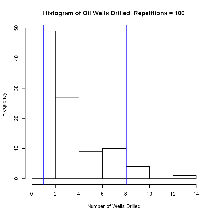
cat('The grand mean of the number of trials needed to achieve success is equal to\n ',mean(num_trials_needed) )
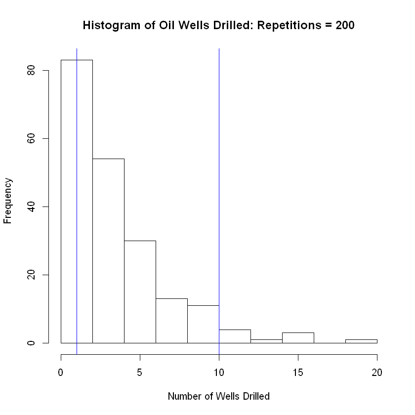
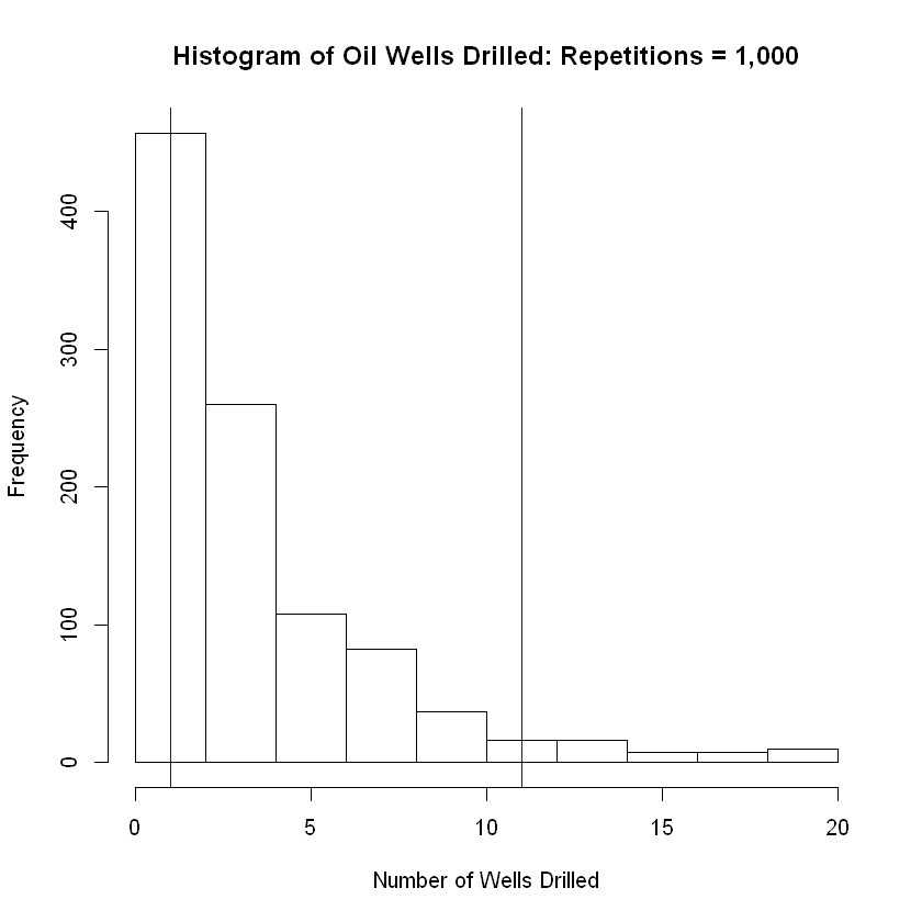
hist(num_trials_needed, breaks = 8, main = 'Histogram of Oil Wells Drilled: Repetitions = 100', xlab = 'Number of Wells Drilled')
abline( v = lower, col="blue") # Add vertical line at 5th percentile
abline(v = upper, col="blue") # Add vertical line at 95th percentile
The grand mean of the number of trials needed to achieve success is equal to
    3.42
This table summarizes the investigation to include five examples from the sampling distribution of Drawing a Spades hand:
| Max Number of Wells Drilled | p = 1/4 | E(X) | Simulation Grand Mean |
|---|---|---|---|
| 100 | 0.25 | 4 | 4.05 |
| 200 | 0.25 | 4 | 3.92 |
| 500 | 0.25 | 4 | 4.28 |
| 1,000 | 0.25 | 4 | 3.857 |