Calculations with the Normal Curve

We some normal distributions for our examples. The following are some well-known distributions.

The SAT has the distribution:

\[N(1000, 200)\]

while the ACT has the distribution:

\[N(21,5)\]

The classic IQ distribution has the distribution:

\[N(100,15)\]

Percentiles

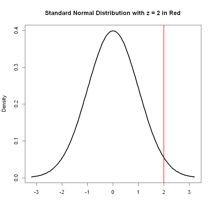
For every z-score we calculate, we can determine the precise percentile. For example, the percentile corresponding to a \(z\)-score of \(z=2\) is given by:

pnorm(2)

0.977249868051821

We can draw the bell curve and resulting standardized score as follows:

x <- seq(-3.2, 3.2, length.out = 100)  # Values along the x-axis.
d <- dnorm(x)                          # Default mean is 0; default sd is 1
plot(x,d, type = 'l',lwd = 3 , main='Standard Normal Distribution with z = 2 in Red', xlab = "",ylab="Density")
abline(v=2, lwd = 2, col="red")

Example 1

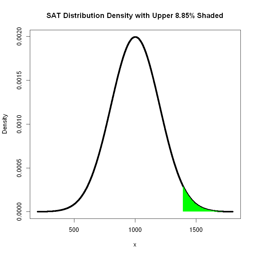
Calculate the \(z\)-score and percentile for someone who scored a 1270 on the SAT. We use the function pnorm() on the \(z\)-score representative of a raw SAT score of 1270:

pnorm((1270-1000)/200)

0.911492008562598

1-0.911492

0.088508

We can add graphics to display the situation. We draw a vertical line at the \(z\)-score, and shade in the tail. The percentile value is \(0.911492\), so the shading is \(1-0.911492 = 0.088508\) or about \(8.85\%\) of the area under the curve.

m = 1000   # Mean of SAT distribution
s = 200    # Standard deviation of SAT distribution
z = (1270 - 1000) / 200            # z-score
x <- seq(m-4*s, m+4*s, by = 0.1)   # x-values for graphing

# Calculate the probability density function
y <- dnorm(x, mean = m, sd = s)
# Plot the results
plot(x, y, type = "l", lwd = 4, main = "SAT Distribution Density with Upper 8.85% Shaded", xlab = "x", ylab = "Density")
# Shade the tail
x2 <- seq(m+1.96*s, m+4*s, length.out = 50)
y <- dnorm(x2, mean = m, sd = s)
polygon(c(x2, m+1.96*s, m+1.96*s), c(y, 0, dnorm(m+1.96*s)), col = "green", border = NA)

Example 2

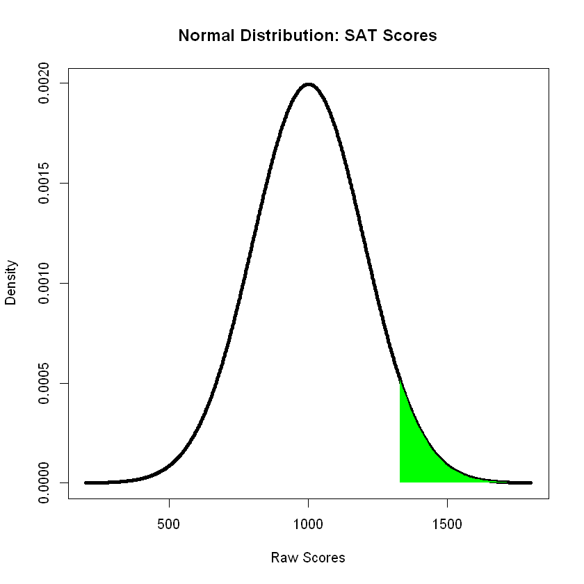
Find the 95th percentile SAT score.

z = qnorm(0.95)
z

1.64485362695147

z = qnorm(0.95)
z

1.64485362695147

SAT = 1000 + 200 * z
SAT

1328.97072539029

We can draw the bell curve indicated with the area under the curve highlighted:

# Generate a sequence of values for the t-distribution
m = 1000   # mean
s = 200    # standard deviation
percent = 0.05
z_left = qnorm(percent)
z_right = qnorm(1-percent)
x <- seq(-4, 4, length = 1000) * s + m

# Calculate the probability density function
y <- dnorm(x, m, s)

# Plot the results
plot(x,y, type = "l", lwd = 4, main = "Normal Distribution: SAT Scores",
     xlab = "Raw Scores", ylab = "Density")
# Left Tail
# x1 <- seq(z_left, -4, length = 50) * s + m
# y1 <- dnorm(x1, m, s)
# polygon(c(x1, m+z_left*s, m+z_left*s), c(y1, 0, dnorm(z_left, m, s)), col = "blue", border = NA)

# Right Tail
x2 <- seq(z_right, 4, length = 50) * s + m
y2 <- dnorm(x2, m, s)
polygon(c(x2, m+z_right*s, m+z_right*s), c(y2, 0, dnorm(z_right, m, s)), col = "green", border = NA)

Example 3

Sally earned a 31 on the ACT while Joanna earned a 1380 on the SAT. Who did better relative to the test she took?

Let’s calculate the \(z\)-score for Sally. Based upon that calculation, we will use the function pnorm() to determine the percentile.

zs = (31 - 21) / 5
zs
pnorm(zs)

2

0.977249868051821

For Joanna, we have a similar calculation:

zj = (1380 - 1000) / 200
zj
pnorm(zj)

1.9

0.971283440183998

We can see that, based upon \(z\)-scores, Sally’s score is 2 standard deviations above the mean relative to the test she took. Joanna’s is only 1.9 standard deviations above the average. However, inspecting the percentiles, we see a very small difference as both were very close to the 97th percentile. Still, Sally’s score is a very slight bit better.

Example 4

What is the 80th percentile IQ score?

We first use the qnorm() to retreive the \(z\)-score for this percentile. Following that, we emplement the \(z\)-score formula to find the actual IQ score correponding to it.

z8 = qnorm(0.8)
z8

0.841621233572914

IQ = 100 + 15 * 0.84
IQ

112.6